Message Boards Message Boards

Save the interpolation function that is a result of NDsolve?

I'm using NSolve to obtain a solution of the nonlinear Schrödinger Equation.

Since the calculations are really time-consuming, I would like to save the results to hard disk for later use. What is an efficient way to save and to load the result of NDsolve, so that I can use the INterpolation function in another notebook?

Thanks you,

Markus

POSTED BY: Markus Schmidt
14 Replies

I have not seen a slow-down within Module, AFAIR. Example:

if = Interpolation@
   Flatten[Table[{{x, t}, Sin[x - t] Cos[x]}, {x, -Pi, Pi, Pi/2.^10}, {t, 0., 5., 1./2^6}], 1];

Module[{},
  Outer[if, Range[-3., 3., 1./8], Range[0., 5., 1./8]];
  ] // AbsoluteTiming
Outer[if, Range[-3., 3., 1./8], Range[0., 5., 1./8]]; // AbsoluteTiming
(*
{0.017717, Null}
{0.017987, Null}
*)
POSTED BY: Michael Rogers

I have tried all the things being suggested, and in the end I create a new 2D matrix (i.e., table) that contains the result of NDsolve at discrete points using the interpolation function (goes along the lines of Neil's suggestion). This is saved and interpolated again and this gives a sufficiently fast response. Thank you all for your suggestions.

What I found out is that if an interpolation function is called from inside a module requires a much longer time than if the same interpolation function is called outside the module. Does anyone has experienced this kind of thing and if yes, how can this be solved?

Best,

M

POSTED BY: Markus Schmidt

I see a problem in choosing the method of integration. It looks like Adams' method is better than others.

L = 50;
Table[{sol = 
   NDSolve[{I D[u[t, x], t] + D[u[t, x], x, x] + 
       2 Abs[u[t, x]]^2 u[t, x] == 0.1 (1 - Cos[Pi x/L]), 
     u[0, x] == Sech[x] Exp[I x], u[t, -L] == u[t, L]}, 
    u, {t, 0, 20}, {x, -L, L}, Method -> m], 
  Plot3D[Evaluate[Abs[u[t, x] /. First[sol]]], {t, 0, 20}, {x, -L, L},
    PlotPoints -> 60, MaxRecursion -> 3, Mesh -> None, 
   ColorFunction -> Hue, PlotRange -> All, 
   PlotLabel -> m]}, {m, {"Adams", "BDF", Automatic}}]

fig

To Michaels point above, I would try using Table to create a 2x2 grid of points, time it, do the FFT on the list of points and see if it is the interpolation that is slowing everything down (and you can control the number of points used this way).

POSTED BY: Neil Singer

The hope with the pseudospectral method is to reduce the size of the spatial grid, which would result in smaller and perhaps faster interpolating function, and to be able to reduce the grid to a size that the time integration does not take too long.

I wonder also if the interpolating function is really that slow, or is it the Fourier transform that is slow.

POSTED BY: Michael Rogers

It's possible to look at the code?

I tried the FunctionInterpolation, but the resulting comparison looks rather bad. Also I'm not sure about the purpose of this function.

I also tried "DifferenceOrder" -> "Pseudospectral". After waiting one hour I stopped the calculations, since no results appear. The only thing which works properly is "DifferenceOrder" ->4.

Really strange.

POSTED BY: Markus Schmidt

Have you tried "DifferenceOrder" -> "Pseudospectral"?

POSTED BY: Michael Rogers

Perfect, I tried Vitaliy's approach and it works. Thanks you all.

Does anyone of you ever had bad experience with the interpolation function generated by NDsolve?

Here is my problem: I have solved the Nonlinear Schrödinger Equation in a more complicated form to analyse ultrafast third harmonic generation in waveguides. The issue is that I have to use a very fine mesh to get the solution, i.e., to get a result which does not show the error message "NDSolve::eerr: Warning: scaled local spatial error estimate of...". The final interpolation function has 6001 steps in spatial and 750 steps in time domain (according to the function shown by Alexander's code) and is extremely slow. The interpolation function is actually so slow that I cannot process the function properly (e.g, to do a numerical FFT). I have no idea how to improve that, i.e., how to make the interpolation function faster.

Is there any trick that speed up the interpolation function (maybe by some option in NDsolve)?

Any help is greatly appreciated.

If anyone has an idea I can provide some code.

M

POSTED BY: Markus Schmidt

Your latter question is interesting (... well, the first as well of course)! Might it be that this is a case for a meaningful application of FunctionInterpolation? - I have never unterstood for what else this function could be useful. What I have in mind is simply like:

easyToEvaluateFunction = FunctionInterpolation[hardToEvaluateFunction[x], {x, x0, x1}];

Or am I completely wrong?

POSTED BY: Henrik Schachner

We can use .txt as well

L = 50;
usol = NDSolve[{I D[u[t, x], t] + D[u[t, x], x, x] + 
     2 Abs[u[t, x]]^2 u[t, x] == 0.1 (1 - Cos[Pi x/L]), 
   u[0, x] == Sech[x] Exp[I x], u[t, -L] == u[t, L]}, 
  u, {t, 0, 1}, {x, -L, L}]
usolE = First[u /. usol]
Export["C:\\Users\\...\\Desktop\\Schrodinger.txt", \
usolE]
Usol = ToExpression[
  Import["C:\\Users\\...\\Desktop\\Schrodinger.txt"]]
In[16]:= Head[Usol]

Out[16]= InterpolatingFunction
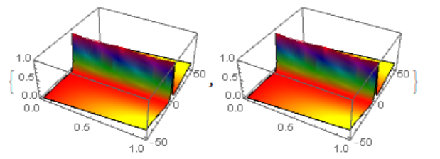
{Plot3D[Abs[usolE[t, x]], {t, 0, 1}, {x, -L, L}, PlotRange -> All, 
  ColorFunction -> Hue, Mesh -> None, PlotPoints -> 50], 
 Plot3D[Abs[Usol[t, x]], {t, 0, 1}, {x, -L, L}, PlotRange -> All, 
  ColorFunction -> Hue, Mesh -> None, PlotPoints -> 50]}

fig

Look up DumpSave and Get.

[Postscript: Vitaliy's answer did not show when the question was loaded. But after I posted my response, there it was.]

POSTED BY: Michael Rogers

The simplest is to use .MX or .WDX formats that store arbitrary Wolfram Language expressions. But MX files cannot be exchanged between operating systems that differ in $SystemWordLength. And MX files created by newer versions of the Wolfram System may not be usable by older

ysol = NDSolveValue[{y'[x] == y[x] Cos[x + y[x]], y[0] == 1}, y, {x, 0, 30}];
Export["ysol.wdx", ysol];
impysol = Import["ysol.wdx"];
Plot[impysol[x], {x, 0, 30}, PlotRange -> All]

enter image description here

POSTED BY: Vitaliy Kaurov
Posted 3 years ago

It is useful but in this way I met a new problem, that is when I save the result with .wdx format, it takes very long time even more than the calculating time, of course the result is very large(maybe several G), and Mathematica quit running automatically, although the local sapce is enough. I hope you can help me to solve it. Thanks!

POSTED BY: Tony Coliderse
Reply to this discussion
Community posts can be styled and formatted using the Markdown syntax.
Reply Preview
Attachments
Remove
or Discard

Group Abstract Group Abstract