WOLFRAM MATERIALS for the ARTICLE:
William Gilpin. Cryptographic hashing using chaotic hydrodynamics.
Proceedings of the National Academy of Sciences, 115 (19) (2018), pp. 4869-4874.
https://doi.org/10.1073/pnas.1721852115
Full article in PDF
Introduction
Last week, William Gilpin published a fascinating paper suggesting a physics-based hashing mechanism in the Proceedings of the National Society: Cryptographic hashing using chaotic hydrodynamics: https://doi.org/10.1073/pnas.1721852115
The paper discusses a hashing algorithm based on fluid mechanics: Particles are distributed in a 2D disk. The inside of the disk is filled with an idealized fluid and the fluid is now stirred with a single stirrer. The stirring process is modelled with two possible stirrer positions. A message (say made from 0s and 1s) can now be encoded through which of the two stirrer positions is active. If the bit from the message is 1, use stirrer position 1, if the bit of the message is 0, use stirrer position 2. After some bites are processed, and the fluid is stirred, this process mixes the particles. Dropping some of the information content of the actual particle positions, e.g. by taking only the x-positions of the particle positions allows to build a hash by using the particle indices after sorting the particles along the x-axis.
The Methods section of the paper mentions that all calculations were carried out using Mathematica 11.0. Unfortunately no notebook supplement was given. So, playing around with ideas of the paper, I re-implemented some of the computations of the paper.
The paper is behind a paywall, but fortunately the author's website has a downloadable copy of the paper here.
The potential importance of physics-based models for hashing, and so for cryptocurrencies was pointed out at various sites (e.g. Stanford News, btcmanager).
It is fun to play around with the model.
The chaotic advection model model
This classic model goes back to Hassan Aref (whom I was fortunate to know personally) from his 1984 paper Stirring by chaotic advection.
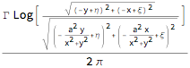
The Hamiltonian for the movement of a particle with coordinates {ξ,η} in a circle of radius a under the influence of agitating vortex at {x,y} (possibly time-dependent) of strength Γ and its mirror vortex.
    H[{ξ_, η_}, {x_, y_}] =
      Γ/(2 π) Log[ComplexExpand[ Abs[((ξ + I η) - (x + I y))/((ξ + I η) - a^2/( x - I y))]] ]
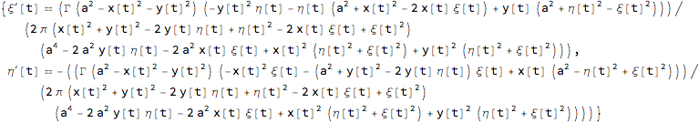
The resulting equations of motion:
odes = {ξ'[t] == -D[H[{ξ[t], η[t]}, {x[t], y[t]}], η[t]],
            η'[ t] == +D[H[{ξ[t], η[t]}, {x[t], y[t]}], ξ[t]]} // Simplify
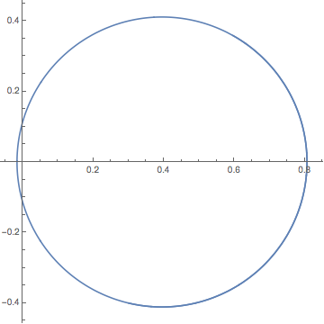
Solve the equations of motion for randomly selected parameters and plot the particle trajectory. For a position-independent and time-independent vortex, the particle moves in a circle.
nds = NDSolveValue[{
   Block[{a = 1, Γ = 1, x = 0.5 &, y = 0 &}, odes],
                 ξ[0] == 0.3, η[0] == -0.4}, {ξ[t], η[t]}, {t, 0, 10}]

ParametricPlot[Evaluate[nds], {t, 0, 10}]
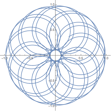
Here the vortex moves around in a periodic manner. The resulting particle trajectory has a high degree of symmetry.
nds2 = NDSolveValue[{
   Block[{a = 1, Γ = 1, x = 0.8 Cos[2 Pi #/200] &, y = 0.8 Sin[2 Pi #/200] &}, odes],
                 ξ[0] == 0.3, η[0] == -0.4}, {ξ[t], η[t]}, {t, 0, 400}]

ParametricPlot[Evaluate[nds2], {t, 0, 400}, PlotPoints -> 400]
Letting the vortex move along a random curve results in a chaotic movement of the particle. We color the particle's trajectory with time.
(* vortex movement curve *)
randomCurve = BSplineFunction[RandomPoint[Disk[], {100}]];

X[t_Real] := randomCurve[t/100][[1]]
Y[t_Real] := randomCurve[t/100][[2]]

nds2 = NDSolveValue[{
   Block[{a = 1, Γ = 10, x = X, y = Y}, odes],
                 ξ[0] == 0.3, η[0] == -0.4}, {ξ[t], η[t]}, {t, 0, 100}]

ParametricPlot[Evaluate[nds2], {t, 0, 100}, PlotPoints -> 1000,
 ColorFunction -> Function[{x, y, u}, ColorData["DarkRainbow"][u]]]
Having two possible positions of the vortex and switching periodically between them results in a particle trajectory that is made of piecewise circle arcs.
nds2 = NDSolveValue[{
    Block[{a = 1, Γ = 10, x = Sign[Sin[Pi #]]/2 &, y = 0 &}, odes],
                  ξ[0] == 2/3, η[0] == 0}, {ξ[t], η[t]}, {t, 0, 100}];

ParametricPlot[Evaluate[nds2], {t, 0, 100}, PlotPoints -> 1000,
 ColorFunction -> Function[{x, y, u}, ColorData["DarkRainbow"][u]]]
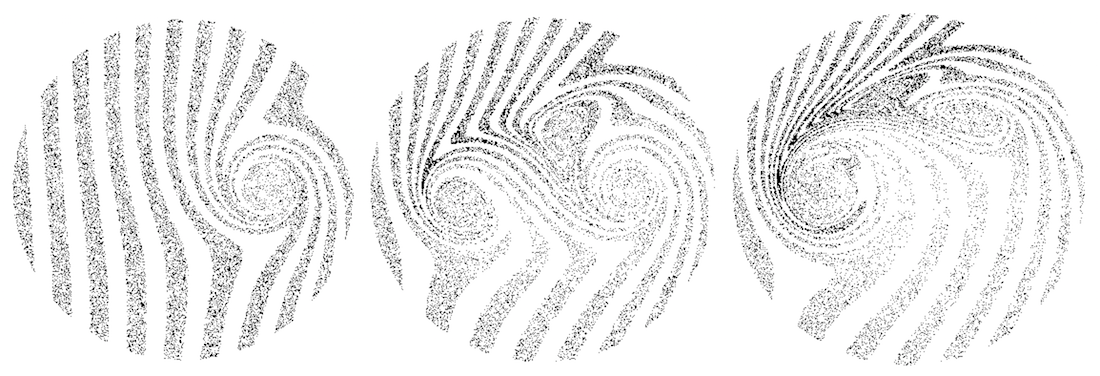
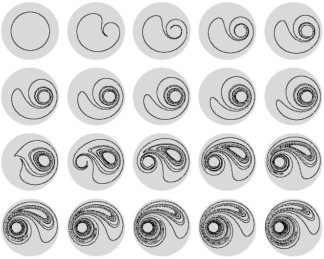
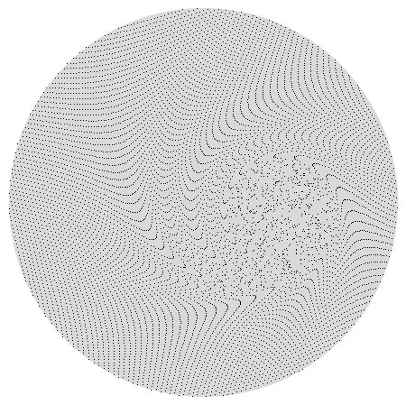
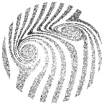
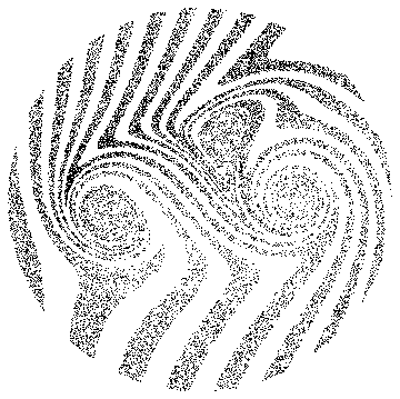
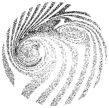
Using initially 4320 points on a circle shows how the initial circle gets stretched and ripped apart and the points distribute chaotically over the disk.
nds2 = NDSolveValue[{
    Block[{a = 1, Γ = 10, x = Sign[Sin[Pi #]]/2 &, y = 0 &}, odes],
                  ξ[0] == Table[2/3 Cos[φ], {φ, 0, 2 Pi, 2 Pi/(12 360)}],
                  η[0] == Table[2/3 Sin[φ], {φ, 0, 2 Pi, 2 Pi/(12 360)}]},
   {ξ[t], η[t]}, {t, 0, 2}];

GraphicsGrid[
 Partition[Graphics[{LightGray, Disk[], Black, PointSize[0.005],
      Point[Transpose[nds2 /. t -> #]]}, ImageSize -> 120] & /@Range[0, 2, 2/19] , 5]]
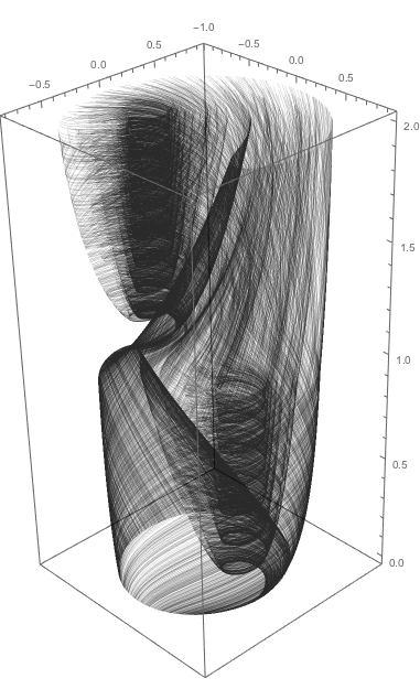
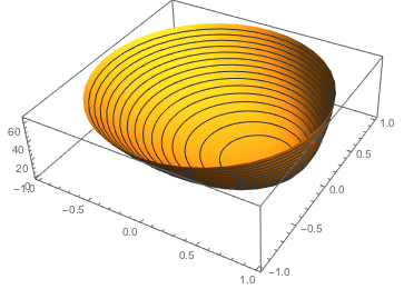
With time running upwards, here is a 3D image of this stirring process. The transition from using the right stirrer to using the left stirrer at time 1 is clearly visible.
trajectories3D =
  Transpose[Table[ Append[#, N[τ]] & /@ Transpose[nds2 /. t -> τ], {τ, 0, 2, 2/100}]];

Graphics3D[{Thickness[0.001], Opacity[0.2],
  BSplineCurve /@ RandomSample[trajectories3D, 1600]},
                          PlotRange -> All, Axes -> True, BoxRatios -> {1, 1, 2}]
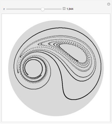
Here is the corresponding interactive demonstration.
Manipulate[
Graphics[{LightGray, Disk[], Black, PointSize[0.005], Point[Transpose[nds2 /. t -> τ]]}],
{τ, 0, 2, Appearance -> "Labeled"}]
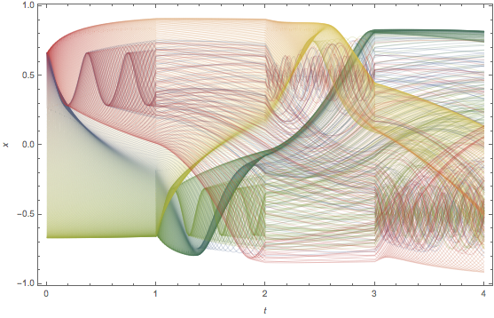
The x-position of the particles will be used later. Here is a plot of the x-positions of 540 points initially on a circle over time.One observes many crossing of these x-trajectories.
nds2B = NDSolveValue[{
    Block[{a = 1, Γ = 4, x = Sign[Sin[Pi #]]/2 &, y = 0 &}, odes],
                  ξ[0] == Table[2/3 Cos[φ], {φ, 0, 2 Pi, 2 Pi/540}],
                  η[0] == Table[2/3 Sin[φ], {φ, 0, 2 Pi, 2 Pi/540}]},
   {ξ[t], η[t]}, {t, 0, 12}];

ListLinePlot[Transpose[Table[{t, #} & /@ nds2B[[1]], {t, 0., 4, 4/200}] ],
 PlotStyle -> Table[Directive[Opacity[0.4], Thickness[0.001], ColorData["DarkRainbow"][j/541]], {j, 541}],
 Frame -> True, Axes -> False, FrameLabel -> {t, x}]
Using a Dynamic[particleGraphics] we can easily model many more particles in real time without having to store large interpolating functions. We solve the the equations of motion over small time increments and the graphic updates dynamically.
rPoints = Select[Flatten[Table[N[{x, y}], {x, -1, 1, 2/101}, {y, -1, 1, 2/101}], 1], Norm[#] < 1 &];

Dynamic[Graphics[{LightGray, Disk[], Black, PointSize[0.001], Point[rPoints]}]]
rhsξ[X_, ξ_List, η_List] := With[{ Γ = 5}, -(((1 - X^2) Γ η (1 + X^2 - 2 X ξ))/(2 π (X^2 + η^2 - 2 X ξ + ξ^2) (1 - 2 X ξ + X^2 (η^2 + ξ^2))))]
rhsη[X_, ξ_List, η_List] := With[{ Γ =  5}, -(((1 - X^2) Γ (-ξ - X^2 ξ +  X (1 - η^2 + ξ^2)))/(2 π (X^2 + η^2 - 2 X ξ + ξ^2) (1 - 2 X ξ + X^2 (η^2 + ξ^2))))]

With[{Δt = 10^-2, T = 0.2},
 Monitor[
  Do[
   nds = NDSolveValue[
      Block[{ X = Evaluate[1/2 Sign[Sin[Pi (k + 1/2) Δt/T]]] &},
               {ξ'[t] == rhsξ[t, ξ[t], η[t]], η'[t] == rhsη[t, ξ[t], η[t]],
                ξ[k Δt] == Transpose[rPoints][[1]],
                η[k Δt] == Transpose[rPoints][[2]]}],
      {ξ[t], η[t]}, {t, (k + 1) Δt, (k + 1) Δt}] /. t -> (k + 1) Δt;
   rPoints = Transpose[nds],
   {k, 0, 200}], k]]
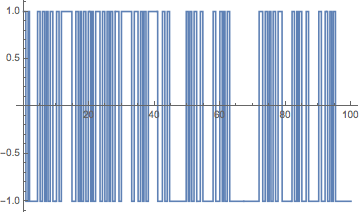
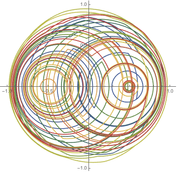
Switching irregularly between the two stirrer positions gives qualitatively similar-looking trajectories. We use a sum of three trig functions see here for a detailed account on this type of function).
(* left or right stirrer is on *)
Plot[Sign[Sin[Pi t] + Sin[Pi Sqrt[2] t] + Sin[Pi Sqrt[3] t]], {t, 0, 100}, Exclusions -> None]
nds3 = NDSolveValue[{
    Block[{a = 1, Γ = 10,
      x = Sign[Sin[Pi #] + Sin[Pi Sqrt[2] #] + Sin[Pi Sqrt[3] #]]/2 &,
      y = 0 &}, odes],    ξ[0] == 2/3, η[0] == 0}, {ξ[t], η[t]}, {t, 0, 100}];

ParametricPlot[Evaluate[nds3], {t, 0, 100}, PlotPoints -> 1000,
 ColorFunction -> Function[{x, y, u}, ColorData["DarkRainbow"][u]]]
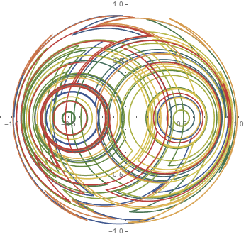
We can also change the stirring direction.
nds3B = NDSolveValue[{
    Block[{a = 1, Γ = 10 Sign[Sin[Pi t] + Sin[Pi Sqrt[2] t] + Sin[Pi Sqrt[3] t]],
      x = Sign[Sin[Pi #] + Sin[Pi Sqrt[2] #] + Sin[Pi Sqrt[3] #]]/2 &,
      y = 0 &}, odes],    ξ[0] == 2/3, η[0] == 0}, {ξ[t], η[
     t]}, {t, 0, 100}];

ParametricPlot[Evaluate[nds3B], {t, 0, 100}, PlotPoints -> 1000,
 ColorFunction -> Function[{x, y, u}, ColorData["DarkRainbow"][u]]]
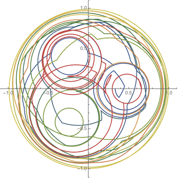
Here are three stirrer positions at the vertices of an equilateral triangle.
st3[t_] = Piecewise[
   With[{r = RandomInteger[{0, 2}]}, {1/2. {Cos[2 Pi r/3], Sin[2 Pi r/3]}, #[[1]] <= t <= #[[2]] }] & /@
    Partition[FoldList[Plus, 0, RandomReal[{0, 1}, 300]], 2, 1]];

x3[t_Real] := st3[t][[1]]
y3[t_Real] := st3[t][[2]]

nds3 = NDSolveValue[{ Block[{a = 1, Γ = 5, x = x3, y = y3}, odes], ξ[0] == 1/3, η[0] == 0}, {ξ[t], η[t]}, {t, 0, 100}]

ParametricPlot[Evaluate[nds3], {t, 0, 100}, PlotPoints -> 1000,
 ColorFunction -> Function[{x, y, u}, ColorData["DarkRainbow"][u]]]
Side note: the linked twist map
Mathematically, alternating left and right use of the stirrer, is isomorphic to a so-called linked twist map. The following implements a simple realization of a linked twist map from Cairns /Kolganova. https://doi.org/10.1088/0951-7715/9/4/011
Clear[g, h, f];
g[{x_, y_}] := {x, Mod[Piecewise[{{y + 4 x, Abs[x] <= 1/4}}, y], 1, -1/2]}
h[{x_, y_}] := {Mod[Piecewise[{{x + 4 y, Abs[y] <= 1/4}}, x], 1, -1/2], y}
f[{x_, y_}] := g[h[{x, y}]]

f[{x, y}]

In explicit piecewise form, the map is more complicated. (To fit it, we use a reduce size.)
(f2 = PiecewiseExpand[# , -1/2 < x < 1/2 && -1/2 < y < 1/2] & /@ f[{x, y}])
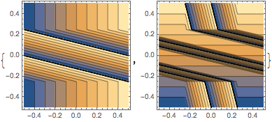
Here are the first and second component visualized.
{ContourPlot[Evaluate[f2[[1]]], {x, -1/2, 1/2} , {y, -1/2, 1/2},
  Exclusions -> {}, PlotPoints -> 60],
 ContourPlot[Evaluate[f2[[2]]], {x, -1/2, 1/2} , {y, -1/2, 1/2},
  Exclusions -> {}, PlotPoints -> 60]}
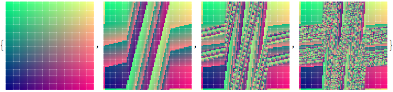
Applying the linked twist map to a set of points inside a square hints at the ergodic nature of the map.
ptsRG = With[{pp = 80}, Table[{RGBColor[x + 1/2, y + 1/2, 0.5], Point[{x, y}]}, {y, -1/2, 1/2, 1/pp}, {x, -1/2, 1/2, 1/pp}]];

Graphics /@ NestList[Function[p, p /. Point[xy_] :> Point[f@xy]], ptsRG, 3]
Closed form mapping
As mentioned, for a fixed stirrer position, a particle moves along a circle. This means that to move the particle to its final position, we don't have to solve nonlinear differential equations, but rather can calculate the final position through algebraic computations which are unfortunately not fully explicit. Doing the calculations (see Aref's paper for details) shows that we will have to solve of transcendental equation.
In the following we will use a unit disk of radius 1 and a unit strength vortex. The particle is initially at {r,θ} (in polar coordinates) and the stirrer is at {±b,0}.
a = 1;
Γ = 1;
The circle the particle is moving on.
circle[{r_, θ_}, b_] :=
 Module[{λ, ξc, ρ},
  λ = Sqrt[(b^2 + r^2 - 2 b r Cos[θ])/(a^4/b^2 + r^2 - 2 a^2 r Cos[θ]/b)];
  ξc = (b - λ^2 a^2/b)/(1 - λ^2);
  ρ = Abs[λ/(1 - λ^2) (a^2/b - b)];
  Circle[{ξc, 0}, ρ]]
The period for one revolution on the circle.
period[{r_, θ_}, b_, T_] :=
 Module[{λ, ρ, Tλ},
  λ = Sqrt[(b^2 + r^2 - 2 b r Cos[θ])/(a^4/b^2 + r^2 - 2 a^2 r Cos[θ]/b)];
  ρ = Abs[λ/(1 - λ^2) (a^2/b - b)];
  Tλ = (2 Pi)^2 ρ^2/Γ (1 + λ^2)/(1 - λ^2) ]
The final position after rotating for time T.
rotate[{r_, θ_}, b_, T_, opts___] :=
Module[{(*λ,ξc,ρ,θp,Tλ,eq,fr*)},
λ = Sqrt[(b^2 + r^2 - 2 b r Cos[θ])/(a^4/b^2 + r^2 - 2 a^2 r Cos[θ]/b)];
ξc = (b - λ^2 a^2/b)/(1 - λ^2);
ρ = Abs[λ/(1 - λ^2) (a^2/b - b)];
θp = ArcTan[r Cos[θ] - ξc, r Sin[θ]];
Tλ = (2 Pi)^2 ρ^2/Γ (1 + λ^2)/(1 - λ^2);
(* the implicit equation to be solved numerically for θt *)

eq = θt - 2 λ/(1 + λ^2) Sin[θt] == θp - 2 λ/(1 + λ^2) Sin[θp] + 2 Pi T/Tλ;
fr = FindRoot[eq, {θt, θp}, opts] // Quiet;  (* could use Solve[eq, θt, Reals] *)
{Sqrt[ρ^2 + ξc^2 + 2 ρ ξc Cos[θt]],
ArcTan[ρ Cos[θt] + ξc, ρ Sin[θt]]} /. fr]
A high-precision version for later use.
 rotateHP[{r_, θ_}, b_, T_ ] :=
 With[{prec = Precision[{r, θ}]},
  rotate[{r, θ}, b, T, WorkingPrecision -> Min[prec, 200] - 1,  PrecisionGoal -> prec - 10]]

rotateHP[{2/5, 1}, 1/2, 10^-10]

{0.3999999999735895736749310453217879335729586969724148186668989989685300449569453838180010833652353802304511654926113687832716502416432363896855780225351918314742068365263060199921670958293439964299441,
1.000000000034865509829422032384759003150106866109371061507406908121303212377635808764825759934117372434662086592066738925787825280696681907390281734196810440241159138906978471624124765879791828431390}
Also for later use, rotate many points at once.
rotate[l : {_List ..}, b_, T_ ] := rotate[#, b, T] & /@ l

rotateHP[l : {_List ..}, b_, T_ ] := rotateHP[#, b, T] & /@ l
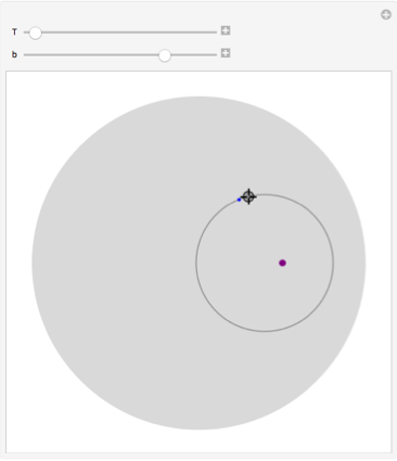
The locator is the initial particle position; the stirrer position is the purple point. We show the circle and the final particle position (gray point).
Manipulate[
 Graphics[{LightGray, Disk[],
   Purple, PointSize[0.02], Point[{b, 0}] ,
   Gray, circle[ToPolarCoordinates[p], b] ,
   PointSize[0.01],
   Point[p], Blue ,
   Point[ FromPolarCoordinates[ rotate @@ SetPrecision[ {ToPolarCoordinates[p], b, T}, 200] ]]}],
 {{T, 0.2}, 0.001, 10},
 {{b, 0.5}, -0.999, 0.999},
 {{p, {0.3, 0.4}}, Locator}]
Here is a plot of the period for one revolution as a function of the initial position of the particle. The period can get quite large when points are near the boundary of the disk
ParametricPlot3D[{r Cos[θ], r Sin[θ], period[{r, θ}, 1/2, 1]},
 {r, 0, 1}, {θ, -Pi, Pi}, BoxRatios -> {1, 1, 0.3},
 PlotPoints -> 40, MeshFunctions -> {#3 &}]
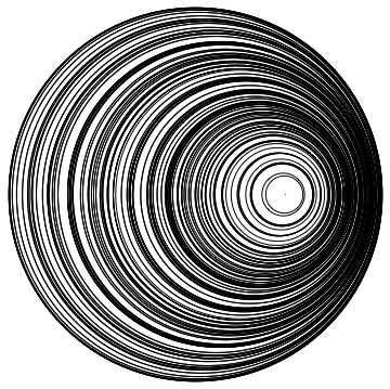
For the stirrer located at {0.5,0}, here are the possible circles that the particle will move on.
Graphics[Table[circle[{r, θ}, 1/2.] , {r, 1/10, 9/10, 1/10}, {θ, -Pi, Pi, 2 Pi/20}]]
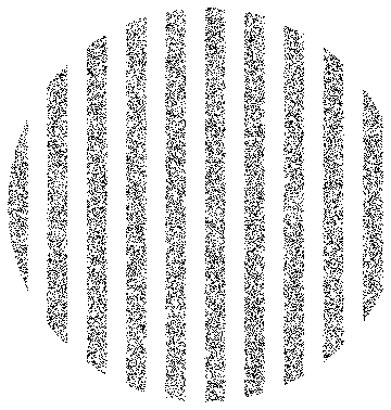
We use the closed form of the stirring map to visualize the flow. Here are about 20k points in stripes in the unit disk.
stripePoints = Select[RandomPoint[Disk[], 40000], Function[xy, Mod[xy[[1]], 0.2] < 0.1]];

Graphics[{PointSize[0.002], Point[stripePoints]}]
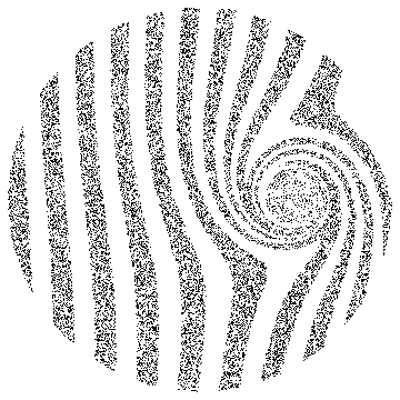
We repeatedly stir with the left and then the right stirrer on for time 1.
swirled[1] = rotate[ToPolarCoordinates[stripePoints], 0.5, 1];

Graphics[{PointSize[0.002], Point[FromPolarCoordinates[swirled[1]]]}]
swirled[2] = rotate[swirled[1], -0.5, 1];

Graphics[{PointSize[0.002], Point[FromPolarCoordinates[swirled[2]]]}]
swirled[3] = rotate[swirled[2], 0.5, 1];

Graphics[{PointSize[0.002], Point[FromPolarCoordinates[swirled[3]]]}]
swirled[4] = rotate[swirled[3], -0.5, 1];

Graphics[{PointSize[0.002], Point[FromPolarCoordinates[swirled[4]]]}]
Now stir and make hashes
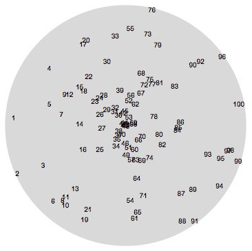
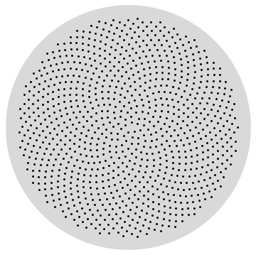
We now use two different initial positions of the points: a sunflower-like one and a random one.
randominitialPositions[n_, prec_] :=
 SortBy[Table[ReIm[RandomReal[{0, 1}, WorkingPrecision -> prec] *
     Exp[ I RandomReal[{-Pi, Pi}, WorkingPrecision -> prec]]], {n}], First]

SeedRandom[1234];
initialPositionsR = randominitialPositions[100, 250];

Graphics[{LightGray, Disk[],
   MapIndexed[Function[{p, pos},
    {Red, PointSize[0.002], Point[p], Black, Text[pos[[1]], p]}],
   N[initialPositionsR]]}]
sunflower[n_, R_, prec_] :=
 Table[FromPolarCoordinates[ N[{Sqrt[j/n] R, Mod[2 Pi (1 - 1/GoldenRatio) j, 2 Pi, -Pi]}, prec]], {j, n}]

Graphics[{LightGray, Disk[], Black, Point[sunflower[1000, 0.9, 20]]}]
The message to encode we will tell in the form of a sequence of 0s and 1s. A zero means use the left stirrer position and a 1 means use the right stirrer position. So, we define a stirring process with a given message σ and fixed b and T as follows:
stirringProcess[initialPositions_, bAbs_, T_, σ_List] :=
  FromPolarCoordinates /@
  FoldList[rotateHP[#1, #2 bAbs, T] &, ToPolarCoordinates /@ initialPositions, 2 σ - 1]
Here is a simple message:
message1 = RandomInteger[{0, 1}, 50]

 {1, 1, 0, 0, 0, 0, 0, 1, 1, 1, 0, 1, 1, 0, 1, 1, 0, 0, 1, 1, 0, 1, 0, 0, 1,
   1, 0, 0, 0, 1, 1, 0, 0, 0, 0, 0, 1, 1, 1, 1, 1, 0, 1, 1, 1, 1,1, 0, 1, 0}
Now we carry out the corresponding stirring process. (We arbitrarily use b=1/2 and T=1/10.)
sP1 = stirringProcess[initialPositionsR, 1/2, 1/10, message1];
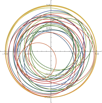
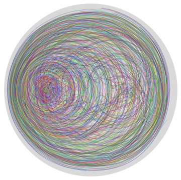
To get a feeling for the stirring process, we connect successive positions of each particle with a randomly colored spline interpolation. (Note that the spline interpolation does not exactly represent the particle's trajectory.)
Graphics[{LightGray, Disk[], Thickness[0.001],
  Map[Function[c, {RandomColor[], BSplineCurve[c, SplineDegree -> 5]}],
   Transpose[N[Table[sP1[[j]], {j, 50}]]]]}]
Now, can we trust these results? We can check by running the stirring process (numerically) backwards.
sP1Rev = stirringProcess[sP1[[-1]], 1/2, -1/10, Reverse[message1]];
The so-recovered initial positions agree to at least 80 digits with the original point positions.
sP1Rev[[-1]] - initialPositionsR // Abs // Max // Accuracy

86.9777
As mentioned earlier, we define the hashes as the positions of the particles when ordered according to their x-values. So, for a given particle configurations, this is the hash-making function.
makeHash[l_] := Sort[ MapIndexed[{#1, #2[[1]]} &, l]][[All, 2]]
Because the hashes are permutations of the particle numberings, the number of hashes grows factorially with the particle number and 58 particles could model a 256 bit hash and 99 particles a 512 bit hash.
{2^256, {57!, 58!}} // N

{1.15792*10^77, {4.05269*10^76, 2.35056*10^78}}

{2^512, {98!, 99!}} // N

{1.34078*10^154, {9.42689*10^153, 9.33262*10^155}}

hashes1 = makeHash /@ sP1;
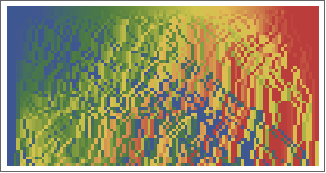
Here is a visualization how the hashes evolve with each stir. The coloring is from blue (1) to 100 (red) of the initial particle numbering.
ArrayPlot[hashes1, ColorFunction -> ColorData["DarkRainbow"], PlotRange -> {1, 100}]
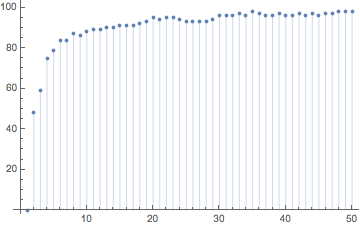
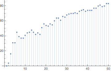
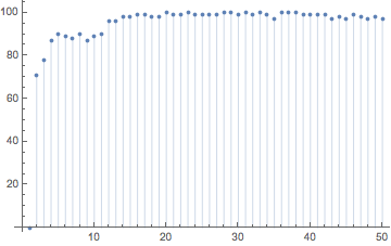
This is how the edit distance of the hashes increases with successive stirrings.
ListPlot[Table[{j, EditDistance[hashes1[[1]], hashes1[[j]]]}, {j, 1, 50}], Filling -> Axis]
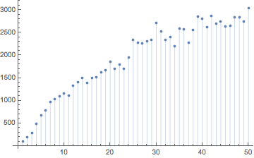
Gilpin defines the rearrangement index of a hash as the sum of the absolute difference between neighboring particle indices.
rearrangementIndex[indexList_] := Total[Abs[Differences[indexList]]]
Here is the growth rate of the rearrangement index for our just-calculated hashes.
ListPlot[Table[{j, rearrangementIndex[hashes1[[j]]]}, {j, 1, 50}], Filling -> Axis]
Let's make a second message that has one bit flipped, say at position 10.
message2 = MapAt[1 - # &, message1, 10]

{1, 1, 0, 0, 0, 0, 0, 1, 1, 0, 0, 1, 1, 0, 1, 1, 0, 0, 1, 1, 0, 1, 0,
 0, 1,  1, 0, 0, 0, 1, 1, 0, 0, 0, 0, 0, 1, 1, 1, 1, 1, 0, 1, 1, 1, 1, 1, 0, 1, 0}

message1 - message2

{0, 0, 0, 0, 0, 0, 0, 0, 0, 1, 0, 0, 0, 0, 0, 0, 0, 0, 0, 0, 0, 0, 0, 0, 0,
0, 0, 0, 0, 0, 0, 0, 0, 0, 0, 0, 0, 0, 0, 0, 0, 0, 0, 0, 0, 0, 0, 0, 0, 0}
The resulting particle movements look quite different.
sP2 = stirringProcess[initialPositionsR, 1/2, 1/10, message2];

Graphics[{LightGray, Disk[], Thickness[0.001],
  Map[Function[c, {RandomColor[], BSplineCurve[c, SplineDegree -> 5]}],
   Transpose[N[Table[sP2[[j]], {j, 50}]]]]}]
The edit distances between the two hash sequences increase quickly after the different bit is encountered.
hashes2 = makeHash /@ sP2;

ListPlot[Table[{j, EditDistance[hashes1[[j]], hashes2[[j]]]}, {j, 0, 50}], Filling -> Axis]
Gilpin carried out many numerical experiments investigating how the hashes behave as a function of the hash length (number of particles), stirring time T, and message length.
The next two examples change only the stirring time, and keep all other parameters: message, stirrer distance, initial particle distance.
sP1B = stirringProcess[initialPositionsR, 1/2, 1/9, message1];

hashes1B = makeHash /@ sP1B;

ListPlot[Table[{j, EditDistance[hashes1[[j]], hashes1B[[j]]]}, {j, 0, 50}], Filling -> Axis]
With increasing stirring time, the edit distance between the hashes quickly increases.
sP1C = stirringProcess[initialPositionsR, 1/2, 1/2, message1];

hashes1C = makeHash /@ sP1C;

ListPlot[Table[{j, EditDistance[hashes1[[j]], hashes1C[[j]]]}, {j, 0, 50}], Filling -> Axis]
Next, we use the phyllotaxis-like initial position from above with 200 particles. We also use a longer stirring time (T=1).
message3 = RandomInteger[{0, 1}, 50]

{0, 1, 0, 0, 1, 0, 0, 0, 0, 1, 0, 1, 0, 1, 0, 0, 0, 1, 1, 1, 0, 1, 1, 1, 1, 0, 0, 0, 1, 0, 1, 1, 0, 0, 1, 1, 0, 0, 1, 1, 1, 1, 1, 0, 0, 0,1, 0, 1, 0}

sP3 = stirringProcess[sunflower[200, 9/10, 250], 1/2, 1, message3];
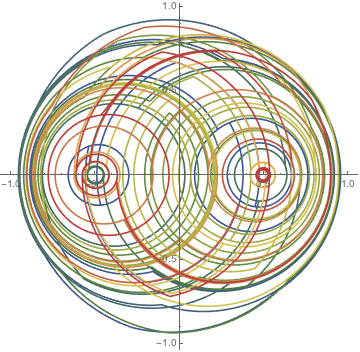
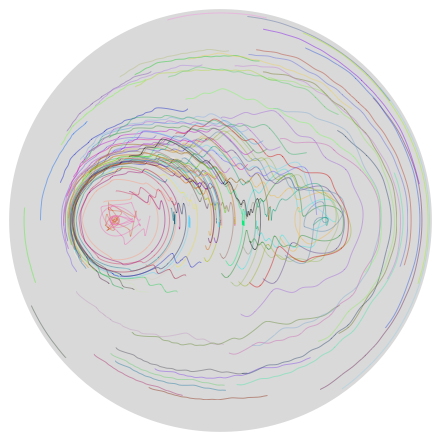
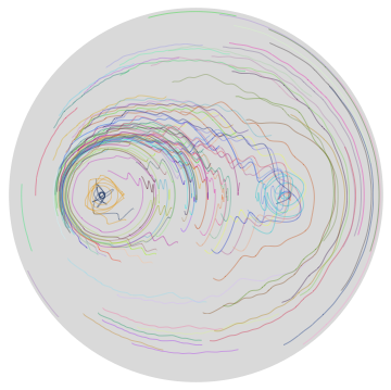
A plot of the 200 particle trajectories suggests a good mixing.
Graphics[{LightGray, Disk[], Thickness[0.001],
  Map[Function[c, {RandomColor[], BSplineCurve[c, SplineDegree -> 5]}],
   Transpose[N[Table[sP3[[j]], {j, 50}]]]]}]
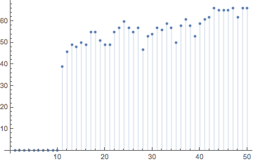
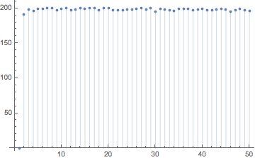
Already after the first stir, the edit distance between the original hash and the one resulting after stirring is quite large.
hashes3 = makeHash /@ sP3;

ListPlot[Table[{j, EditDistance[hashes3[[1]], hashes3[[j]]]}, {j, 0, 50}], Filling -> Axis]
We will end here. The interested reader can continue to model, stir a million times, count trajectory exchanges, and statistically analyze other aspects of the proposed hashing scheme from Gilpin's paper.
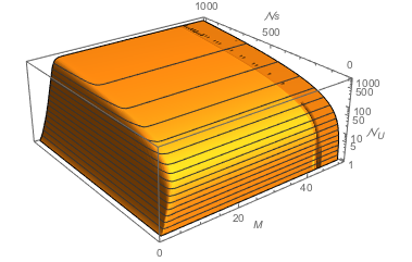
PS: And one can compare with theoretical hashing probabilities for ideal hashes. Such as: draw [ScriptCapitalN]s hashes from M! possible hashes. How many different hashes Subscript[[ScriptCapitalN], U] does one draw in average?
uniqueHashes[M_, \[ScriptCapitalN]s_] :=
 M! (1 - (1 - 1/M!)^\[ScriptCapitalN]s)

Plot3D[uniqueHashes[M, \[ScriptCapitalN]s], {M, 1, 60}, {\[ScriptCapitalN]s, 1, 1000}, MeshFunctions -> {#3 &},
 PlotPoints -> 100, ScalingFunctions -> "Log", PlotRange -> All,
 WorkingPrecision -> 50,
 AxesLabel -> {Style["M", Italic], Style["\[ScriptCapitalN]s", Italic], Style["\!\(\*SubscriptBox[\(\[ScriptCapitalN]\), \(U\)]\)", Italic]}]
For Ns≪M!, this becomes:
Series[Mfac (1 - (1 - 1/Mfac)^\[ScriptCapitalN]s), {Mfac, ∞, 2}] /. Mfac -> M! // Simplify
uniqueHashesApprox[M_, \[ScriptCapitalN]s_] := \[ScriptCapitalN]s - (\[ScriptCapitalN]s*(\[ScriptCapitalN]s - 1))/(2*M!) + (\[ScriptCapitalN]s*(\[ScriptCapitalN]s - 1)*(\[ScriptCapitalN]s - 2))/(6*M!^2)
Here is a quick numerical modeling with a sample size of 100 from 6!=720 possible hashes.
With[{M = 6, \[ScriptCapitalN]s = 100},
  {Table[Length[
      Tally[RandomChoice[Range[M!], \[ScriptCapitalN]s]]], {10000}] // Mean,
   uniqueHashes[M, \[ScriptCapitalN]s],
   uniqueHashesApprox[M, \[ScriptCapitalN]s]}] // N

{93.407, 93.4267, 93.4369}
I definitely suggest reading the whole paper, including the Supplementary Information.
The notebook with all the code and visualizations is attached.
 Attachments:


