Message Boards Message Boards

Solve ODE system with BVP?

Posted 6 years ago

I have a system of 3 non-linear ODEs of 2nd order with 3 unknown functions and 6 boundary conditions at Pi. I need to find functions numerically, get their plots and then calculate an integral containing these 3 functions. First is the system: I tried solving it with NDSolve but it gives me an error (NDSolve::ndsz: At x == 1.9672446444378016`, step size is effectively zero; singularity or stiff system suspected.) and the plots are wrong. I solved this system in Maple earlier so I think I'm making some syntax mistake since I'm not very familiar with Wolfram... Here's my code:

a = -10^2; b = 1; c = -2*10^(-3); m = 10^(-2); Rpi = 10^(-3); mupi = 4; Ypi = 10^(-2);
system = {R0''[x] + R0'[x]*Cot[x] == Exp[2*mu[x]]/2*((R0[x])^2 - c/a - m^2*(Y0[x])^2/a), R0[x]*Exp[2*mu[x]] == 2*(1 - mu''[x] - mu'[x]*Cot[x]), Y0''[x] + Y0'[x]*Cot[x] - m^2*Exp[2*mu[x]]*Y0[x] == 0, R0[Pi] == Rpi, R0'[Pi] == 0, mu[Pi] == mupi, mu'[Pi] == 0, Y0[Pi] == Ypi, Y0'[Pi] == 0}
sol = NDSolve[system, {R0, mu, Y0}, {x, 0, Pi}]
Plot[Evaluate[R0[x] /. sol], {x, 0, Pi}, PlotRange -> All]

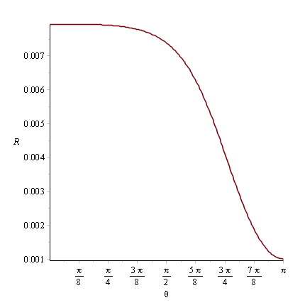
What am I doing wrong? I know that a cot(x) can create a singularuty, but only at 0 or Pi, not at 1.97... On Maple plots there are singularities at 0 and that's fine, but not in R(x):

enter image description here

POSTED BY: Aaeru Michi
9 Replies

I changed the sign of parameter $a$ and added options in NDSolve. Apparently, the parameters should be selected more carefully to exit the singular point.

a = 10^2; b = 1; c = -2*10^(-4); m = 10^(-2); Rpi = 
10^(-3); mupi = 4; Ypi = 10^(-2);
system = {R0''[x] + R0'[x]*Cot[x] == 
Exp[2*mu[x]]/2*((R0[x])^2 - c/a - m^2*(Y0[x])^2/a), 
R0[x]*Exp[2*mu[x]] == 2*(1 - mu''[x] - mu'[x]*Cot[x]), 
Y0''[x] + Y0'[x]*Cot[x] - m^2*Exp[2*mu[x]]*Y0[x] == 0, 
R0[Pi] == Rpi, R0'[Pi] == 0, mu[Pi] == mupi, mu'[Pi] == 0, 
Y0[Pi] == Ypi, Y0'[Pi] == 0};
sol = NDSolveValue[system, {R0, mu, Y0}, {x, 0, Pi}, 
Method -> {"StiffnessSwitching", "NonstiffTest" -> False}] // 
Quiet;
Plot[sol[[1]][x], {x, 0., Pi}, PlotRange -> All, 
AxesLabel -> {\[Theta], R}] // Quiet

fig1

Can you show the original system of equations?

You solve numerically then better is use NIntegrate than Integrate. The correct syntax is:

R1[x] = Evaluate[sol[[1]][x]];
mu1[x] = Evaluate[sol[[2]][x]];
Y1[x] = Evaluate[sol[[3]][x]];
Y2[x] = Evaluate[D[sol[[3]][x], x]];
NIntegrate[Sin[x]*Exp[2*mu1[x]]*(a*(R1[x])^2 + b*R1[x] + c - (Y2[x])^2/2/Exp[2*mu1[x]] - m^2/2*(Y1[x])^2), {x, 0, Pi},WorkingPrecision -> 20]
(* 9.0569457332837941551 *)
POSTED BY: Mariusz Iwaniuk

Now we can calculate the integral (Sorry Mariusz, we changed the system of equations and parameters):

In[57]:= NIntegrate[
 Sin[x]*Exp[
   2*sol[[2]][x]]*(a*(sol[[1]][x])^2 + b*sol[[1]][x] + 
    c - (sol[[3]]'[x])^2/2/Exp[2*sol[[2]][x]] - 
    m^2/2*(sol[[3]][x])^2), {x, 0, Pi}]

Out[57]= 0.128767
Posted 6 years ago

It's x instead of theta, doesn't really matter...

enter image description here

POSTED BY: Aaeru Michi
Posted 6 years ago

Thanks a lot! I realized a mistake in signs in equations and got a correct answer thanks to you. enter image description here

Now I need to integrate some expression numerically, I hope you can help. Or should I create another discussion? Basically I need to integrate this:

Integrate[Sin[x]*Exp[2*mu[x]]*(a*(R0[x])^2+b*R0[x]+c-(Y0'[x])^2/2/Exp[2*mu[x]]-m^2/2*(Y0[x])^2), {x, 0, Pi}]

And in this case I don't know a correct answer because Maple doesn't seem to work with this kind of integral correctly. I'm not sure how to "get" solutions from sol to put them into the integral, like this maybe:

R1[x] = Evaluate[R0[x] /. sol]
mu1[x] = Evaluate[mu[x] /. sol]
Y1[x] = Evaluate[Y0[x] /. sol]
Y2[x] = Evaluate[Y0'[x] /. sol]
Integrate[Sin[x]*Exp[2*mu1[x]]*(a*(R1[x])^2+b*R1[x]+c-(Y2[x])^2/2/Exp[2*mu1[x]]-m^2/2*(Y1[x])^2), {x, 0, Pi}]

But it doesn't really help: Wolfram gives me errors and doesn't calculate it...

POSTED BY: Aaeru Michi

Now it looks like in Maple

a = -10^2; b = 1; c = -2*10^(-4); m = 10^(-2); Rpi = 
 10^(-3); mupi = 4; Ypi = 10^(-2);
system = {R0''[x] + 
     R0'[x]*Cot[x] == -Exp[2*mu[x]]/
      2*((R0[x])^2 - c/a - m^2*(Y0[x])^2/a), 
   R0[x]*Exp[2*mu[x]] == 2*(1 - mu''[x] - mu'[x]*Cot[x]), 
   Y0''[x] + Y0'[x]*Cot[x] - m^2*Exp[2*mu[x]]*Y0[x] == 0, 
   R0[Pi] == Rpi, R0'[Pi] == 0, mu[Pi] == mupi, mu'[Pi] == 0, 
   Y0[Pi] == Ypi, Y0'[Pi] == 0};
sol = NDSolveValue[system, {R0, mu, Y0}, {x, 0, Pi}, 
    Method -> {"StiffnessSwitching", "NonstiffTest" -> False}] // 
   Quiet;
Plot[sol[[1]][x], {x, 0., Pi}, PlotRange -> All, 
  AxesLabel -> {\[Theta], R}, PlotRange -> All] // Quiet

fig

Posted 6 years ago

Thank you, you totally helped me!

POSTED BY: Aaeru Michi
Posted 6 years ago

Thank you once more!

POSTED BY: Aaeru Michi
Reply to this discussion
Community posts can be styled and formatted using the Markdown syntax.
Reply Preview
Attachments
Remove
or Discard

Group Abstract Group Abstract