MODERATOR NOTE: a submission to computations art contest, see more: https://wolfr.am/CompArt-22
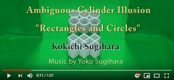
Intrigued by the Ambiguous Cylinder Illusion, of prof. Kokichi Sugihara, I started looking for explanations with the help of Wolfram Language.
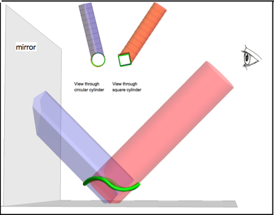
The "ambiguous cylinder" can, for purposes of the viewing illusion, be reduced to its upper rim. We call the rim an "ambiguous ring". This ring can be seen as a circle or a square, depending on the viewpoint. Almost perpendicular, viewpoints can be achieved with the help of a mirror.
Looking parallel to the axis of the circular cylinder or of the square cylinder (prism) will show a circle or a square respectively. A possible mathematical expression for this "ambiguous curve" can be obtained by investigating the intersection of a circular with a square cylinder. My Wolfram demonstrations Intersection of Circular and Polygonal Cylinders 1] and [Ambiguous Rings 1: Polygon Based illustrate the different intersection curves obtained by changing the geometry of the cylinders. For these intersection curves to form a ring, a tight fit between the square cylinder inside the circular one is required. The circumradius of a perfectly fitted square inside a circle of radius 1 is:
fittedradius4[t_] :=
 Module[{n}, n = 2 Floor[4 (.5 t + \[Pi]/8)/\[Pi]] - 1;
  Cos[t - (n + 1) \[Pi]/4]]
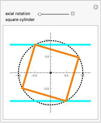
As can be seen in this simple Manipulate:
Manipulate[
 ParametricPlot[
  1/Sqrt[2] Sec[
    1/2 ArcTan[Cot[2 (\[Theta] - \[Theta]0)]]] {Cos[\[Theta]],
    Sin[\[Theta]]}, {\[Theta], 0, 2 \[Pi]},
  PlotStyle -> Directive[AbsoluteThickness[4], Orange],
  PlotRange -> 1.25, ImageSize -> Small, TicksStyle -> 6,
  Prolog -> {{Thick, Dotted, Circle[]}, Cyan, AbsoluteThickness[4],
    Line[{{-5, fittedradius4[\[Theta]0]}, {5,
       fittedradius4[\[Theta]0]}}],
    Line[{{-5, -fittedradius4[\[Theta]0]}, {5, \
-fittedradius4[\[Theta]0]}}], AbsolutePointSize[5], Black,
    Point[{0, 0}]}],
 {{\[Theta]0, 0.5, "axial rotation\nsquare cylinder"}, 0, 10 \[Pi],
  ImageSize -> Tiny}, TrackedSymbols :> Manipulate]
Based on [1], this is the function for a polygonal ringset:
polyRingsetCF =
Compile[{{\[Theta], _Real}, {r, _Real}, {\[Theta]0, _Real}, {d, \
_Real}, {n, _Integer}, {\[Alpha], _Real}},
Module[{t},
t = Sec[2 ArcTan[Cot[1/2 n (\[Theta] - \[Theta]0)]]/
n]; {(*part1*){Cos[\[Pi]/n] Cos[\[Theta]] t,
Cos[\[Pi]/n] t Sin[\[Theta]],
Sec[\[Alpha]] Sqrt[-d^2 + r^2 +
2 d Cos[\[Pi]/n] t Sin[\[Theta]] -
Cos[\[Pi]/n]^2 t^2 Sin[\[Theta]]^2] -
Cos[\[Pi]/n] Cos[\[Theta]] t Tan[\[Alpha]]},
{(*part 2*)Cos[\[Pi]/n] Cos[\[Theta]] t,
Cos[\[Pi]/
n] t Sin[\[Theta]], -Sec[\[Alpha]] Sqrt[-d^2 + r^2 +
2 d Cos[\[Pi]/n] t Sin[\[Theta]] -
Cos[\[Pi]/n]^2 t^2 Sin[\[Theta]]^2] -
Cos[\[Pi]/n] Cos[\[Theta]] t Tan[\[Alpha]]}}]];
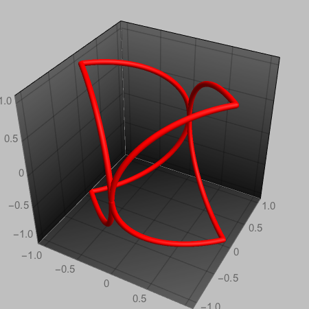
ParametricPlot3D[
polyRingsetCF[t, 1., 0.5, 0., 4, 0.], {t, -\[Pi], \[Pi]},
PlotStyle -> {{Red, Tube[.035]}}, PlotPoints -> 500,
PerformanceGoal -> "Quality", SphericalRegion -> True,
PlotRange -> 1.1, Background -> Lighter[Gray, 0.5], ImageSize -> 300,
PlotTheme -> "Marketing"]
If we now use fittedRadius[[Theta]0] as the circumradius for the square cylinder, we can create closed ringsets as a function the axial rotation [Theta]0 of the suare cylinder. This is a GIF scrolling through all possible fitted square cylinders inside a circular cylinder of radius 1 :
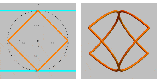
These intersection curves are composite curves (ringsets) consisting each of two separate curves (rings). We can select one of these two rings by introducing the cutoff angles (t1 and t2) in the parametric plot [2].
polyRingCF =
Compile[{{\[Theta], _Real}, {\[Theta]0, _Real}, {r, _Real}, \
{\[Alpha], _Real}, {n, _Integer}, {d, _Real}, {t1, _Real}, {t2, \
_Real}},(*t1 and t2 are the values of \[Theta] for switching between \
parts*)
Module[{t},(*selection of parts of a composite curve*)
t = Sec[2 ArcTan[Cot[1/2 n (\[Theta] - \[Theta]0)]]/n];
{Cos[\[Pi]/n] Cos[\[Theta]] t,
Cos[\[Pi]/n] Sin[\[Theta]] t,(*select part1 or part 2*)
Piecewise[{{1, \[Theta] <= t1 \[Pi] + 2 \[Theta]0 || \[Theta] >
t2 \[Pi] + 2 \[Theta]0}}, -1]*(Sec[\[Alpha]] Sqrt[-d^2 +
r^2 + 2 d Cos[\[Pi]/n] t Sin[\[Theta]] -
Cos[\[Pi]/n]^2 t^2 Sin[\[Theta]]^2]) -
Cos[\[Pi]/n] Cos[\[Theta]] t Tan[\[Alpha]]}]]
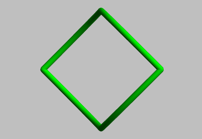
printring4 =
ParametricPlot3D[
polyRingCF[\[Theta], 0., fittedradius4[0.], 0., 4,
0., -.5, .5], {\[Theta], -\[Pi], \[Pi]}, SphericalRegion -> True,
PlotStyle -> {Green, Tube[.05]}, Boxed -> False, Axes -> False,
PlotRange -> 1.05, PlotPoints -> 100, ImageSize -> Small,
PlotTheme -> "ThickSurface"]
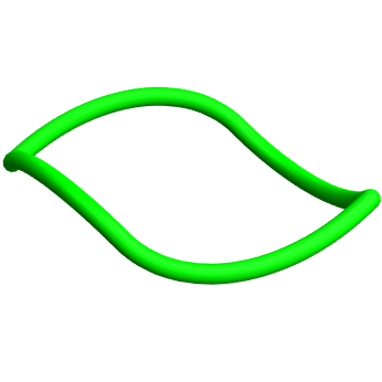
This is a GIF showing the different views of this ring: among them a circle, a square, a "lemniscate", etc...
To test this "ambiguous ring" in a mirror setup, we use Printout3D to send the file to Sculpteo for 3D-printing:
Printout3D[printring4, "Sculpteo", RegionSize -> Quantity[5, "cm"]]
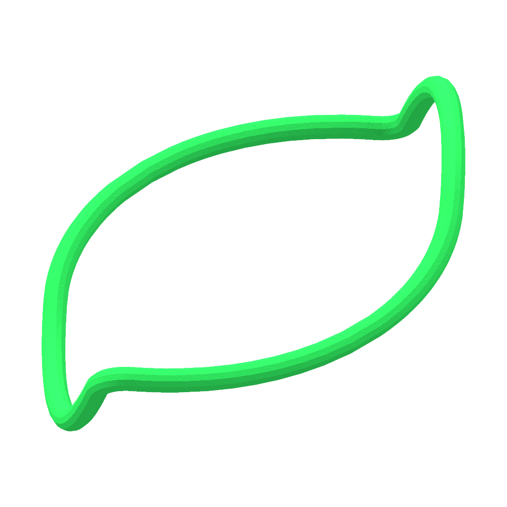
And when reflected in an experimental mirror setup: 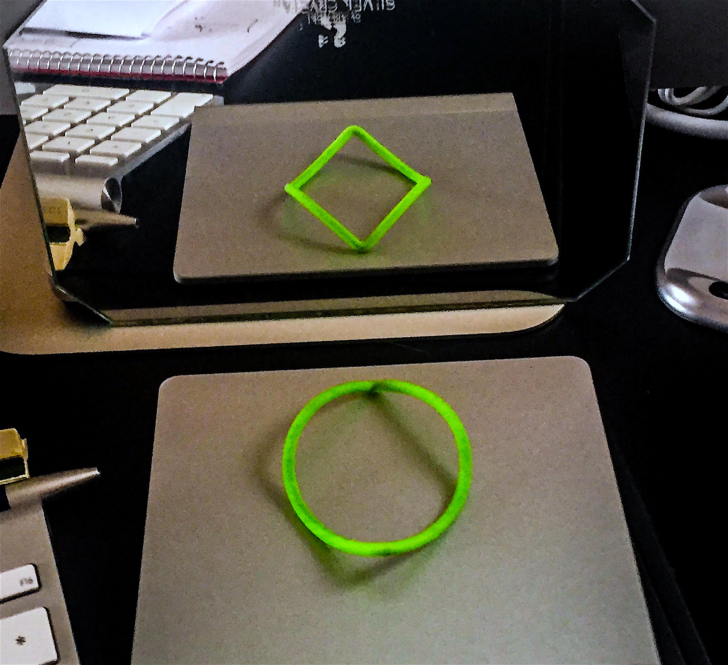
The physical ring looks like a circle while the reflected ring looks like a square.
For those who like to print this ring themselves, This is the link to the Sculpteo file.


