Message Boards Message Boards

Heat Transfer Problem

Posted 11 years ago
Hi, im currently trying to work on the following formulae for a 1-d transient Heat transfer problem.


Basically it is a bar with 2 ends where each end has a fixed temperature after t=0 meaning to say that one end is being heated while the other is cooled to a fixed temperature. i want to get a sketch of temp vs time and the solution for dT/dt

my boundary condtions are
T(0,0)=301K=T(L,0)
and when it reaches steady state at an unknown time, 
T(0,t)=293
T(L,t)=473

so with L = 5 i tried solving the equation but i kept coming up with the same error.

heatsol =
NDSolve[{3.25D[temp[x, t], t] == -0.0000447D[
temp[x, t], {x, 2}], temp[0, 0] == 301, temp[5, 0] == 301,
temp[5, t] == 473}, temp, {x, 0, 5}, {t, 0, 100}]


NDSolve::deqn: Equation or list of equations expected instead of True in the first argument {3.24776 (temp^(0,1))[x,t]==-0.000044705 (temp^(2,0))[x,t],temp[0,0]==301,temp[5,0]==301,True,temp[0,t]==273}. >>

but if i assigned a random number to the boundary condition where it reaches steady state, temp[5,100] i get the following error saying that my initial condition is redundant

heatsol =
NDSolve[{3.247755102 D[temp[x, t], t] == -0.000044705030299999997 D[
temp[x, t], {x, 2}], temp[5, 0] == 301, temp[5, 100] == 473},
temp, {x, 0, 5}, {t, 0, 100}]


NDSolve::bcedge: Boundary condition temp[5,0]==301 is not specified on a single edge of the boundary of the computational domain. >>
POSTED BY: Jon T
10 Replies
Posted 11 years ago
@Shenghui

1. Both ends are heated/cooled via conduction. so i was wondering if i need to co-relate another transient state equation to the boundary conditions(governed by the heat transfer equation through the respective heating/cooling blocks) 

2. Is it possible to use the piecewise function to follow a similar gradient to dTemp/dtime as shown in the formula? because i don't think the actual transient condition is a linear path. 

also 

besides using the function 
Manipulate[
Plot[Evaluate[temp[x, t] /. sol], {t, 0, 100},
  PlotRange -> Full], {x, 0, 5}]
 is it possible to plot a 2D graph of (temp,time) showing at x= 0 and 5 on 1 plot,
i couldnt seem to get it using the plot function
Plot[Evaluate[temp[x, t] /. sol, [0, t]], {t, 0, 100},
PlotRange -> {Automatic, {270, 480}}]


thanks for all your help! i've learnt quite abit!
POSTED BY: Jon T
@Jon

1. If they are both heated gradually, you will need to append two conduction process to this model aka the beam is no longer with uniform thermal property

2. The result really depends on the time scale of transient process. You can in most cases use linear approximation for a system at transient state if 1) peak value is not a big deal and  2) raise time (10% -> 90% of steady state) is relatively short and 3) the response is almost monotonic (or oscillation plays no role). I think linearization should make sense here. Your request may involve some effor beyond the purpose of this forum

3. You just need: 
Plot[{Evaluate[temp[x1, t] /. sol],Evaluate[temp[x2, t] /. sol]}, {t, 0, 100},<options sit here>]
POSTED BY: Shenghui Yang
Posted 11 years ago
@Shenghui

Hmm.. I'm still trying to learn how Mathematica sees this problem.

Because solving it analytically, i just need 
a PDE, IC and BC.
But in Mathematica i need to approixmate the the gradient at 0 and L which i thought the PDE would solve.

Do you think if i change the boundary conditions to T(0,t)=473 from t>5 to infinity would it work without using the linear approximation in the piecewise function?
Also is there a way to input a function that allows me to put a boundary coundition say t>0 without specifiying it through the piecewise function

or how do i specify such boundary condition too.
T(0,0)=273
T(5,0)=473
but at the same time,from x=0.5 to x= 4.5 it is T(x,0)=293
POSTED BY: Jon T
The documentation page of NDSolve talks about this type of problem. Go to "Basic Example" -> The 4th example. 
POSTED BY: Shenghui Yang
Posted 11 years ago
@Jon,

I too am interested in solving this class of partial differntial equation problem..

If you are still having trouble solving this, you might consider "zooming-out" and find a "textbook" solution on the web to a similar problem and see if you can coax Mathematica to solve it.  Since you would know the solution ahead of time you could compare it to what Mma gives you. Then if you still have trouble you could point us to the known solution along with your attempt at solving it. This way, the boundary conditions and all other details would be clearly defined, consistent and visible to others. Once you/we learn how to solve the textbook problem it should be a snap to jump to your/our real problem.
POSTED BY: Steve M
@Jon, 

1. I do not think so. Since the numeric solution depends upon the raise time of the temperature at two ends, the actual process of heating or cooling the two ends are necessary. 

2. I think they are same here: 

3. From your screenshot it seems that "temp" is with a definition (since the font color is black instead of blue). Please run
Clear[temp]
and then try again. 
POSTED BY: Shenghui Yang
Posted 11 years ago
@shenghui & Steve

okay so to link it to the practical experiment, the time should be dependent on how long the heater and cooler.

so since the heating is produce by a voltage source and the cooling by a refrigerant, how do i tag the conditions of the heater and cooler to the boundary conditions of this problem? say because it is a transient response from when i start the 2 devices  but i am only concerned with the fixed temperature of which it reaches steady state.

However, to find this time to acheive steady state, it must first be calculated by another set of equations. should i be using a transient formulae or a steady state one and how do i tag this time to reach steady state to the boundary condition for the above equation.

Thanks!
POSTED BY: Jon T
@Jon, 

Then I suggest two ways: 

1. Do the experient to find the approximation 
or 
2. Include a boundary layer of thin air. This thin layer/thermal resistor is responsible for the heat loss/gain via convection. So the beam is not uniform in terms of thermal parameters. 
POSTED BY: Shenghui Yang
Posted 11 years ago
Hi Shenghui,


Thank you for your reply,


There are 3 things that i would like to clarify,

1. is it possible to solve this if i do not know the heating time as i am just applying the heat at both ends and waiting for the rod to reach those temperatures at its respective ends.

2. As i'm still new and learning mathematica, 
sol = NDSolve[{
   3.25 D[temp[x, t], t] == 0.0447 D[temp[x, t], x, x],
   temp[0, t] == f1[t],
   temp[5, t] == f2[t],
   temp[x, 0] == 301
   }, temp, {x, 0, 5}, {t, 0, 100}, MaxStepFraction -> 1/20]
 why is it such that for dˆ2T/dxˆ2 the function is written as temp[x,t],x,x instead of temp[x,t],{x,2}. from what i understand from the help file, {x,2} is the 2nd order and x,x is dT/dxdx so i'm reather confused here.

3. also, after inputting the script above, i get an error even after establishing the f1 and f2 before this.


once again thanks alot for your help but as i'm still learning the software, your further clarification would help me understand.
POSTED BY: Jon T
@Jon, 

These boundary conditions do not like each other: 
temp[5, 0] == 301
temp[5, t] == 47
Even the evolvement of the temperature is not known, it is required to define such process instead of using arbitary abrupt change here. 

Here is a modification of your system: (Coefficients are adjusted for better visualization):
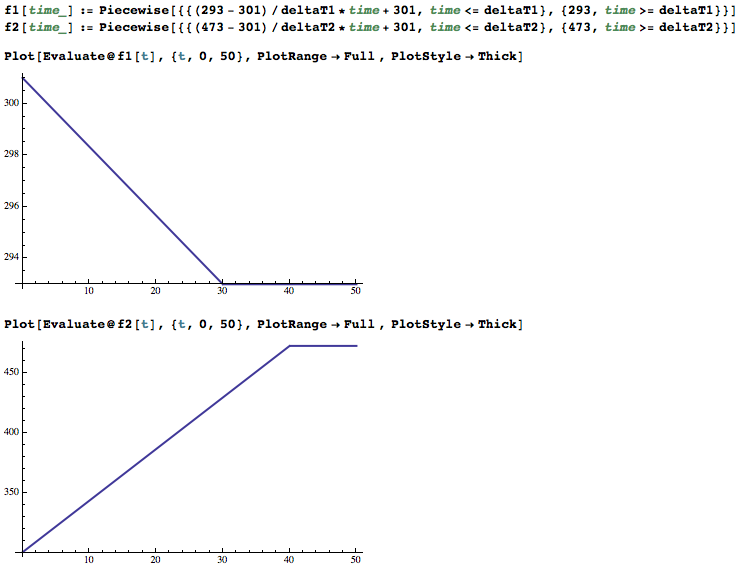
lets assume that we know the time used for heating up and cooling down both ends. You can adjust them later
deltaT1 = 30;
deltaT2 = 40;
Then I use the piecewise function here to approximate thermal exchange processes at two ends with first order: 
f1[time_] := Piecewise[{{(293 - 301)/deltaT1*time + 301, time <= deltaT1}, {293, time >= deltaT1}}]
f2[time_] := Piecewise[{{(473 - 301)/deltaT2*time + 301, time <= deltaT2}, {473, time >= deltaT2}}]

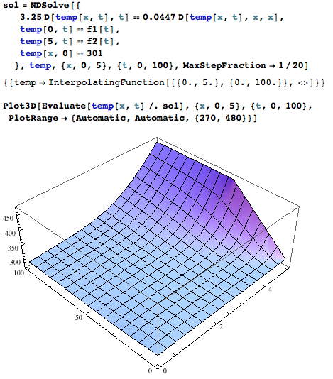
Once I have these steps specified, I can find how the 1-d rod respond to the time-dependent temperature profile at its two ends:
sol = NDSolve[{
   3.25 D[temp[x, t], t] == 0.0447 D[temp[x, t], x, x],
   temp[0, t] == f1[t],
   temp[5, t] == f2[t],
   temp[x, 0] == 301
   }, temp, {x, 0, 5}, {t, 0, 100}, MaxStepFraction -> 1/20]
Plot3D[Evaluate[temp[x, t] /. sol], {x, 0, 5}, {t, 0, 100},
PlotRange -> {Automatic, Automatic, {270, 480}}]

With Manipulate function, I can visualize the evolvement of the thermal system over 100 time steps
Manipulate[
DensityPlot[
  Evaluate[temp[x, t] /. sol], {x, 0, 5}, {y, -0.02, 0.02},
  ColorFunction -> (ColorData["TemperatureMap"][#1] &),
  PlotRange -> {{0, 5}, {-0.01, 0.01}, {270, 480}},
  PlotLegends -> Automatic, AspectRatio -> 0.1, MaxRecursion -> 3,
  FrameTicks -> {Automatic, None}],
{t, 0, 100}]


POSTED BY: Shenghui Yang
Reply to this discussion
Community posts can be styled and formatted using the Markdown syntax.
Reply Preview
Attachments
Remove
or Discard

Group Abstract Group Abstract