Introducing Hadamard Binary Neural Networks

Deep neural networks are an important tool in modern applications. It has become a major challenge to accelerate their training. As the complexity of our training tasks increase, the computation does too. For sustainable machine learning at scale, we need distributed systems that can leverage the available hardware effectively. This research hopes to exceed the current state of the art performance of neural networks by introducing a new architecture optimized for distributability. The scope of this work is not just limited to optimizing neural network training for large servers, but also to bring training to heterogeneous environments; paving way for a distributed peer to peer mesh computing platform that can harness the wasted resources of idle computers in a workplace for AI.

Network Architecture and Layer Evaluator

Here, I will describe the network and the Layer Evaluator, to get an in depth understanding of the network architecture.

Note:

• hbActForward : Forward binarization of Activations.

• hbWForward : Forward binarization of Weights.

• binAggression : Aggressiveness of binarization (Vector length to binarize)

Set up the Layer Evaluator.

layerEval[x_, layer_Association] := layerEval[x, Lookup[layer, "LayerType"], Lookup[layer, "Parameters"]];
layerEval[x_, "Sigmoid", param_] := 1/(1 + Exp[-x]);
layerEval[x_, "Ramp", param_] := Abs[x]*UnitStep[x];
layerEval[ x_, "LinearLayer", param_] := Dot[x, param["Weights"]];
layerEval[ x_, "BinLayer", param_] := Dot[hbActForward[x, binAggression], hbWForward[param["Weights"], binAggression]];
layerEval[x_, "BinarizeLayer", param_] := hbActForward[x, binAggression];
netEvaluate[net_, x_, "Training"] := FoldList[layerEval, x, net];
netEvaluate[net_, x_, "Test"] := Fold[layerEval, x, net];

Define the network

net = {<|"LayerType" -> "LinearLayer", "Parameters" -> <|"Weights" -> w0|>|>,
          <|"LayerType" -> "Ramp"|>,
          <|"LayerType" -> "BinarizeLayer"|>,
          <|"LayerType" -> "BinLayer", "Parameters" -> <|"Weights" -> w1|>|>, 
          <|"LayerType" -> "Ramp"|>,
          <|"LayerType" -> "BinLayer", "Parameters" -> <|"Weights" -> w2|>|>, 
          <|"LayerType" -> "Sigmoid"|>       };

MatrixForm@netEvaluate[net, input[[1 ;; 3]], "Test" ] (* Giving network inputs *)

Advantages of Hadamard Binarization

• Faster convergence with respect to vanilla binarization techniques.
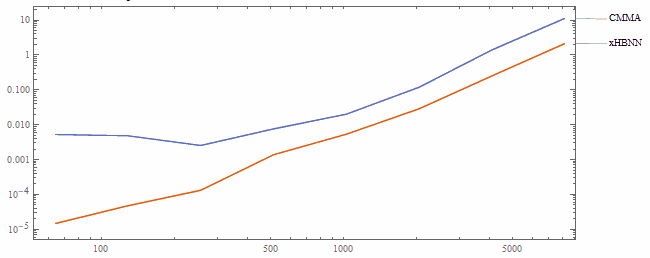
• Consistently about 10 times faster than CMMA algorithm.
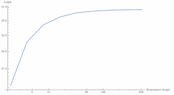
• Angle of randomly initialized vectors preserved in high dimensional spaces. (Approximately 37 degrees as vector length approach infinity.)
• Reduced communication times for distributed deep learning.
• Optimization of im2col algorithm for faster inference.
• Reduction of model sizes.

Accuracy analysis

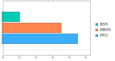
As seen above, the HBNN model gives 87% accuracy, whereas the BNN model (Binary Neural Networks) give only 82%. These networks have only been trained for 5 epochs.

Performance Analysis

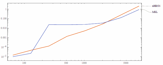
X Axis: Matrix Size | Y Axis: Time (seconds)

CMMA vs xHBNN

MKL vs xHBNN

$\hspace{1mm}$

Visualize weight histograms

It is evident that the Hadamard BNN preserves the distribution of the weights much better. Note that the BNN graph has a logarithmic vertical axis, for representation purposes.

Demonstration of the angle preservation ability of the HBNN architecture

Binarization approximately preserves the direction of high dimensional vectors. The figure above demonstrates that the angle between a random vector (from a standard normal distribution) and its binarized version converges to ~ 37 degrees as the dimension of the vector goes to infinity. This angle is exceedingly small in high dimensions.