What is Spectroscopy?

Each element in the universe has a unique signature given by a sequence of wavelengths or frequencies that can be represented by spectral lines. These lines are equivalent to the transition energy between atomic orbitals; that is, the energy an electron needs to emit or absorb to move to different energy levels.

Why is this relevant?

These unique signatures can tell us a lot about the properties of an element. But perhaps a more interesting application of spectroscopy is the fact that it can tell us about the chemical composition of a light source by matching the lines in its spectrum to the lines of known elements. This applies to spectra of stars, galaxies, planets, atmospheres and more, and it can be especially useful for remote sensing, astrophysics, and planetary sciences.

Spectral Analysis with Machine Learning

The basic idea of spectral analysis is to take the spectrum of the light source we are interested in studying and matching it with known elements. This can be easily done with an algorithm that runs the spectrum through every possible signature and combination. Sounds simple enough. However, we have 118 elements, each with different levels of ionization, and an extremely big number of possible combinations. This means the identification process using an algorithm is slow. The machine learning approach to the problem makes it much simpler and gives you a match almost instantly.

How to choose the appropriate data set

The goal of this project was to create a spectral analysis tool in Wolfram Language and be as broad as possible without losing accuracy due to unnecessary data. Only 90 out of 118 chemical elements occur naturally in the universe. The abundance of elements in the universe also serves as a guideline for the expected common combinations and compounds. Hydrogen is the most abundant element and makes up 75% of the universe, followed by 23% of Helium, 1% of Oxygen, and 0.5% of Carbon.

The Process

Part 1

The first step is to generate enough spectra using the wavelength data available through the built-in function SpectralLineData. Random noise is generated and added to each line value. The added noise is two orders of magnitude bigger than the precision in the original data, which should be enough to account for quantum broadening of the lines and other general measurement uncertainty. Thread is used to associate the wavelengths to the corresponding element. The process should be repeated at least 100 times for each element and ion. Once that data is produced and saved, the tables of spectra with random noise can be combined to form compounds.

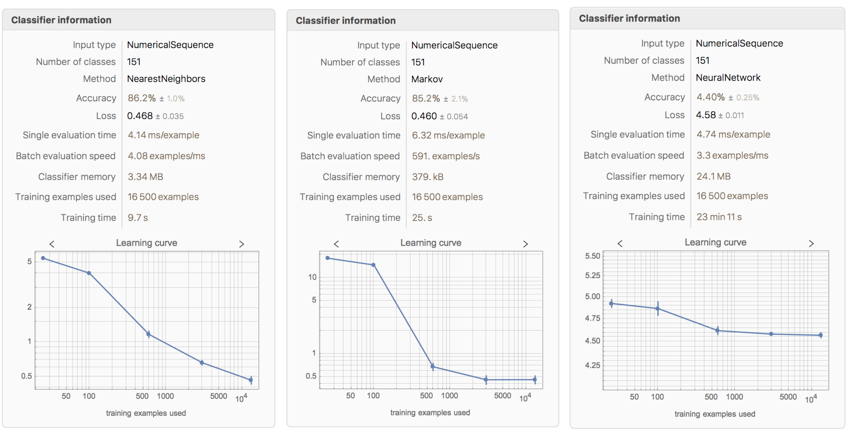
The complete data set is created by joining all element, ion, and compound tables. The data set is then used to train Classify. The classifier function is called elementClassify. The total number of classes for the wavelength data is 151. The function takes 1min 28s to train and the accuracy is 86.2% when using the NearestNeighbors method. The following methods are also tested: DecisionTree, GradientBoostedTrees, LogisticRegression, Markov, NaiveBayes, NeuralNetwork, RandomForest, and SupportVectorMachine. Most of them exhibit slightly lower accuracy than NearestNeighbors, but still show above 84% success. NeuralNetwork and SupportVectorMachine both perform poorly, exhibiting less than 4% accuracy.

The code is shown below.

(* linedata generates spectral lines for element "elem" and ionization level "ion" *)

linedata[elem_, ion_] := 
  Part[{lines = 
      SpectralLineData[
       EntityClass[
        "AtomicLine", {elem, ion}], {Quantity[300.000, "Nanometers"], 
        Quantity[800.000, "Nanometers"]}];, 
    wavelength = 
     QuantityMagnitude[SpectralLineData[lines, "Wavelength"], 
      "Nanometers"]}, 2];

(* iongenerate generates "n" (numerical) spectra with random noise of element "elem" and ionization level "ion" and matches them 
with the corresponding element *)

iongenerate[elem_, ion_, n_] := 
  Thread[Table[linedata[elem, ion] + RandomReal[0.1], n] -> 
    elem <> " " <> RomanNumeral[ion]];

(* here, elem1 and elem2 are tables of two different elements made using iongenerate, mixgenerate takes the two tables and creates
a compound *)

mixgenerate[elem1_, elem2_] := 
  Part[{wdata = 
      Table[Flatten[Join[{elem1[[i, 1]], elem2[[i, 1]]}]], {i, 1, 
        100}];,
    ldata = 
      Flatten[
       Table[{elem1[[1, 2]] <> "-" <> elem2[[1, 2]]}, {i, 1, 100}]];, 
    compounds = Thread[wdata -> ldata]}, 3];

Part 2

Once the wavelength classifier function is trained, the next step is to train a classifier on the images of the spectra. Data is again generated using SpectralLineData and random noise is added to the lines. Thread is used for the element associations. Again, compounds can be generated by combining tables of pure elements. The complete data set is created by joining all element, ion, and compound tables. The data is saved and used to train the classifier function on the images. The classifier function is called spectrumClassifyThe total number of classes is 140. The function takes 9min 41s to train and the accuracy is 97.2% when using the LogisticRegression method. No other methods are tested due to time constraints.

The code is shown below

(* spectrumgenerate generates "n" (visual) spectra with random noise of element "elem" and ionization level "ion" and matches them
with the corresponding element *)

spectrumgenerate[elem_, ion_, n_] := 
  Thread[Table[
     Part[{lines = 
         SpectralLineData[
          EntityClass[
           "AtomicLine", {elem, ion}], {Quantity[300.000, 
            "Nanometers"], Quantity[800.000, "Nanometers"]}];, 
       wavelength = 
         QuantityMagnitude[SpectralLineData[lines, "Wavelength"], 
           "Nanometers"] + RandomReal[0.1];, 
       Graphics[{ColorData["VisibleSpectrum"][#], 
           Line[{{#, 0}, {#, 1}}]} & /@ wavelength, 
        AspectRatio -> 1/6.5, Background -> Black]}, 3], n] -> 
    elem <> " " <> RomanNumeral[ion]];

(* here, elem1, elem2, etc. are tables of different elements generated using spectrumgenerate, spmix takes these tables and
creates compounds of up to 8 elements. This can be increased by adding more arguments to the function *)

spmix[elem1_, elem2_] := 
  Thread[Show[elem1[[1, 1]], elem2[[1, 1]]] -> 
    elem1[[1, 2]] <> ", " <> elem2[[1, 2]]];
spmix[elem1_, elem2_, elem3_] := 
  Thread[Show[elem1[[1, 1]], elem2[[1, 1]], elem3[[1, 1]]] -> 
    elem1[[1, 2]] <> ", " <> elem2[[1, 2]] <> ", " <> elem3[[1, 2]]];
spmix[elem1_, elem2_, elem3_, elem4_] := 
  Thread[Show[elem1[[1, 1]], elem2[[1, 1]], elem3[[1, 1]], 
     elem4[[1, 1]]] -> 
    elem1[[1, 2]] <> ", " <> elem2[[1, 2]] <> ", " <> elem3[[1, 2]] <>
      ", " <> elem4[[1, 2]]];
spmix[elem1_, elem2_, elem3_, elem4_, elem5_] := 
  Thread[Show[elem1[[1, 1]], elem2[[1, 1]], elem3[[1, 1]], 
     elem4[[1, 1]], elem5[[1, 1]]] -> 
    elem1[[1, 2]] <> ", " <> elem2[[1, 2]] <> ", " <> elem3[[1, 2]] <>
      ", " <> elem4[[1, 2]] <> ", " <> elem5[[1, 2]]];
spmix[elem1_, elem2_, elem3_, elem4_, elem5_, elem6_] := 
  Thread[Show[elem1[[1, 1]], elem2[[1, 1]], elem3[[1, 1]], 
     elem4[[1, 1]], elem5[[1, 1]], elem6[[1, 1]]] -> 
    elem1[[1, 2]] <> ", " <> elem2[[1, 2]] <> ", " <> elem3[[1, 2]] <>
      ", " <> elem4[[1, 2]] <> ", " <> elem5[[1, 2]] <> ", " <> 
     elem6[[1, 2]]];
spmix[elem1_, elem2_, elem3_, elem4_, elem5_, elem6_, elem7_] := 
  Thread[Show[elem1[[1, 1]], elem2[[1, 1]], elem3[[1, 1]], 
     elem4[[1, 1]], elem5[[1, 1]], elem6[[1, 1]], elem7[[1, 1]]] -> 
    elem1[[1, 2]] <> ", " <> elem2[[1, 2]] <> ", " <> elem3[[1, 2]] <>
      ", " <> elem4[[1, 2]] <> ", " <> elem5[[1, 2]] <> ", " <> 
     elem6[[1, 2]] <> ", " <> elem7[[1, 2]]];
spmix[elem1_, elem2_, elem3_, elem4_, elem5_, elem6_, elem7_, 
   elem8_] := 
  Thread[Show[elem1[[1, 1]], elem2[[1, 1]], elem3[[1, 1]], 
     elem4[[1, 1]], elem5[[1, 1]], elem6[[1, 1]], elem7[[1, 1]], 
     elem8[[1, 1]]] -> 
    elem1[[1, 2]] <> ", " <> elem2[[1, 2]] <> ", " <> elem3[[1, 2]] <>
      ", " <> elem4[[1, 2]] <> ", " <> elem5[[1, 2]] <> ", " <> 
     elem6[[1, 2]] <> ", " <> elem7[[1, 2]] <> ", " <> elem8[[1, 2]]];

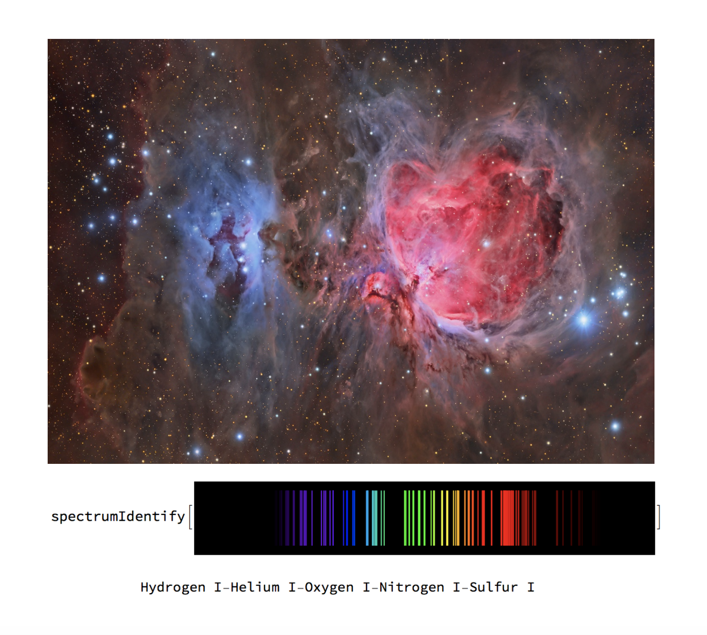
Finally, an identification function is created to accept both numerical sequences and images as the input and runs it through the appropriate classifier function. The output is the chemical composition of the input.

The code is shown below

(* spectrumIdentify tests if the input is a list. If yes, it uses elementClassify to identify the composition. If not, it uses
spectrumClassify. Give "max" to get top probabilities *)

spectrumIdentify[input_, max_] := 
 If[ListQ[input], elementClassify[input, "TopProbabilities" -> max], 
  spectrumClassify[input, "TopProbabilities" -> max]]

The Learning Curve of Different Methods

Confusion Matrix

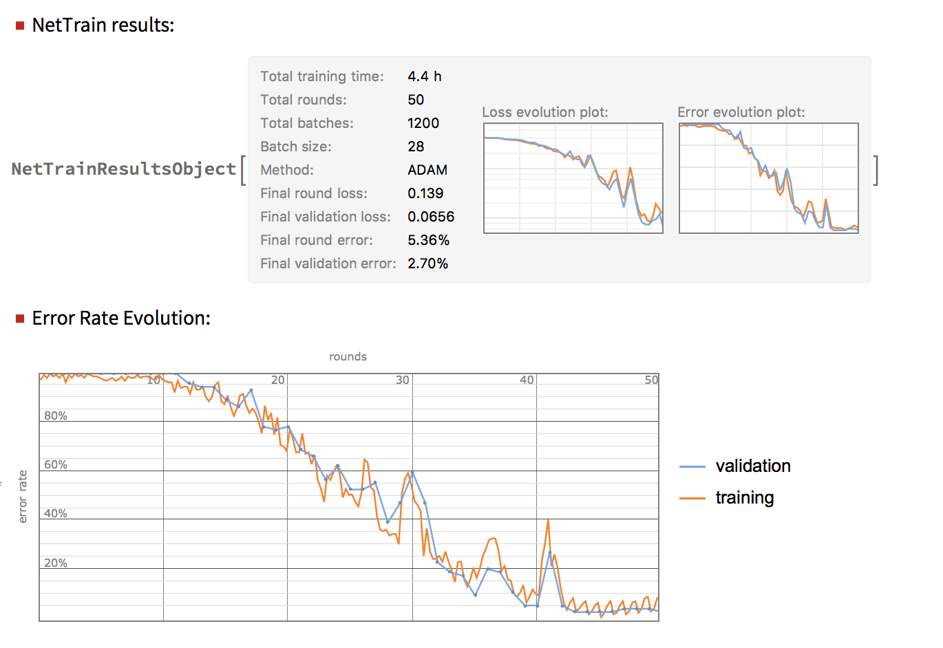
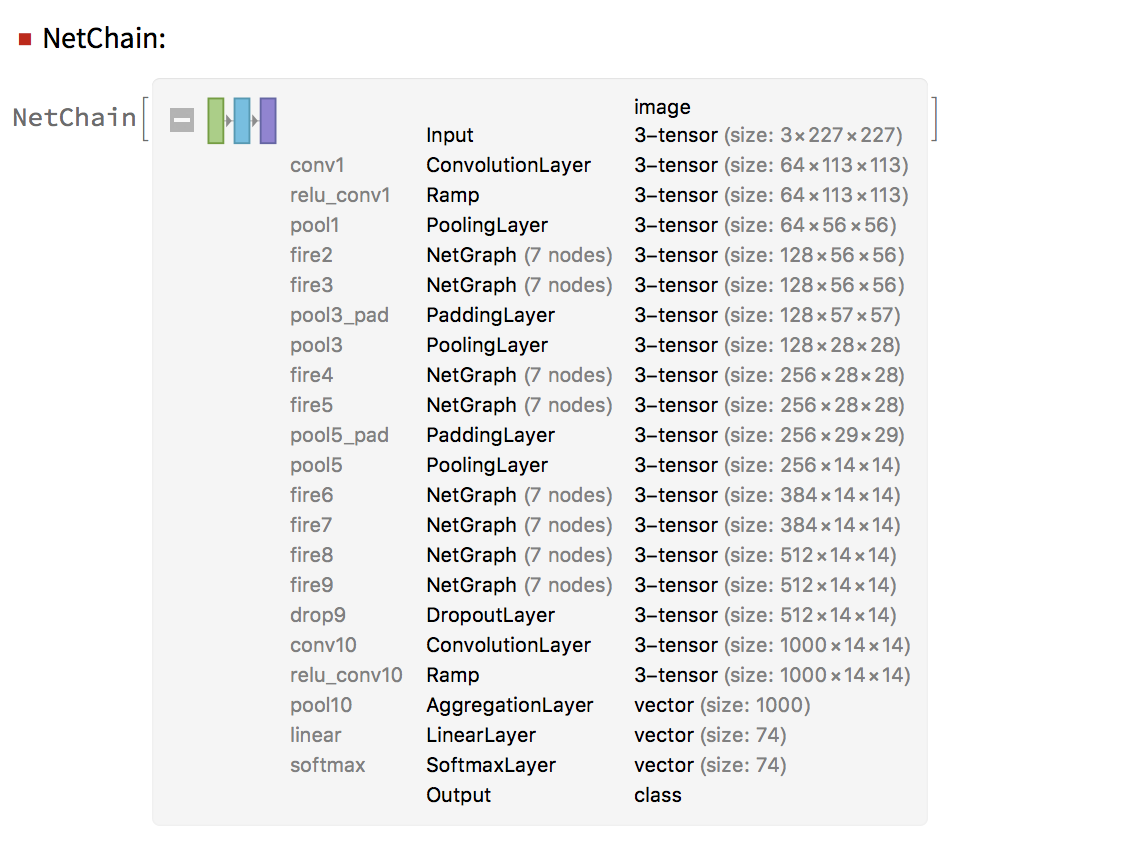
Neural Network for Spectral Classification

Neural networks can give a slightly better accuracy than LogisticRegression for the spectral images if trained for long enough. The results can be seen below.

Conclusion and Future Work

The classifier trained on images performs much better than the classifier trained on the numerical sequence of wavelengths. But either way, using machine learning for spectral analysis is much more efficient than other methods that are currently being used, such as compressed sensing, because it is relatively easy to train a function on spectral data, the accuracy is good, and it is way faster to test a sample and to find a match than it would be to run an algorithm through all of the possibilities.

In the future, the classifier function can be expanded to support more ions and combinations, and accuracy can be improved by training Classify on more data samples. The Process section of this post offers a step-by-step of how to create the spectrum classifier function, and can be reproduced to generate more data, add it to the existent data and retrain the classifier. The classifier is trained on highly accurate and detailed data, so it does not work very well with lower definition spectra. This can be improved by adding lower definition data to the classifier. It can also be expanded to account for Doppler shifting, which is very useful for investigating the motion of light sources and has several astrophysical and cosmological applications. Image manipulation can also be implemented to expand the classifier's ability to determine the chemical composition from absorption spectra and perhaps have an option to identify if the input is an emission spectrum or an absorption spectrum.

References

Condon, E. U., & Shortley, G. (1999). The theory of atomic spectra. New York: Cambridge University Press.

Ralchenko, Y., et al. "NIST Atomic Spectra Database (Version 4.0.1)." National Institute of Standards and Technology

Sobel?man, I. I. (1996). Atomic spectra and radiative transitions. Berlin: Springer.

https://www.nist.gov/pml/atomic-spectra-database