Introduction
This project aims to create a neural network agent that plays Atari games. This agent is trained using Q-Learning. The agent will not have any priori knowledge of the game. It is able to learn by playing the game and only being told when it loses.
What is reinforcement learning?
Reinforcement learning is an area under the general machine Learning, inspired by behavioral psychology. The agent learns what to do, given a situation and a set of possible actions to choose from, in order to maximize a reward. Therefore, to model a problem to reinforcement learning problem, the game should have a set of states, a set of actions that able to transfer one state into another and a set of reward corresponding to each state. The mathematical formulation of reinforcement learning problem is called Markov Decision Process (MDP). 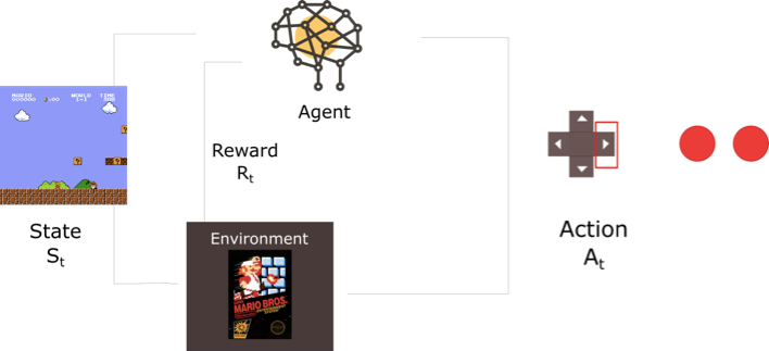 Image From:https://medium.freecodecamp.org/diving-deeper-into-reinforcement-learning-with-q-learning-c18d0db58efe
Markov Decision Process
Before apply Markov decision process to the problem, we need to make sure the problem satisfy the Markov property which is that ?the current state completely represents the state of the environment. For short, the future depends only on the present. An MDP can be defined by (S,A,R,P,?) where:
- S??set of possible states
- A??set of possible actions
- R??probability distribution of reward given (state, action) pair
- P??probability distribution over how likely any of the states is to be the new states, given (state, action) pair. Also known as transition probability.
- ???reward discount factor
At initial state $S_{0}$, the agent chooses action $A_{0}$. Then the environment gives reward $R_{0}=R(.|S_{0}, A_{0})$ and next state $S_{1}=P(.|S_{0},A_{0})$. Repeats till the environment ends.
Value Network
In value-based RL, the input will be the current state or a combination of few recent states, and the output will be the estimated future reward of every possible action at this state. The goal will be to optimize the value function so that the prediction value is close to the actual reward. In the following graph, each number in the box represents the distance from current box to the goal.
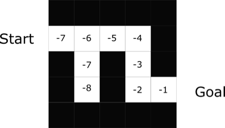
Image From:https://medium.freecodecamp.org/diving-deeper-into-reinforcement-learning-with-q-learning-c18d0db58efe
Deep Q-Learning
Deep Q-learning is the algorithm that I used to construct my agent. The basic idea of Q function is to get the state and action then output the corresponding sum of rewards till the end of the game. In deep Q-learning, we use a neural network as the Q function therefore we can use one state as input and let neural network to generate the prediction for all possible actions. The Q function is stated as following.
$Q(S_{t},A) = R_{t+1}+\gamma maxQ(S_{t+1},A)\\Where:\\Q(S_{t},A)\,\,\,\,\,\,\,\,\,\,\,\,\, = The \,predicted\,sum \,of rewards \,given\, current\,state\,and\,selected\,action\\R_{t+1} \,\,\,\,\,\,\,\,\,\,\,\,\,\,\,\,\,\,\,\,\,= Reward\,received\,after\,taking\,action\\\gamma \,\,\,\,\,\,\,\,\,\,\,\,\,\,\,\,\,\,\,\,\,\,\,\,\,\,\,\,\,= Discount\,factor\\maxQ(S_{t+1},A) = The\,prediction\,of\,next\,state$
As we can see that given current state and action, Q function outputs the reward of current plus the max value of the predictions of next state. This function will iteratively predicts the reward till the end of the game where Q[S,A] = R. Therefore we can calculate the loss by minus the prediction of current state with the sum of the reward and the prediction of the next state. When loss equals to 0, the function will able to perfectly predicts the reward of all actions. In another sense that the Q function is predicting the future value of its own prediction. People might ask how could this function be ever converge? Yes, this function is usually hard to converge but when it converges, the performance is really well. There are a lot of techniques that can be used to speed up the converge of the Q function. I will talk about a few techniques I used in this project.
Experience Replay
Experience replay means that the agent will remember the states that it has experienced and learn from those experience when training. It gives more efficient way of using generated data which is by learning it for multiple times. It is important when gaining experience is expensive to agent. Since the Q function usually don't converge in a short time which means a lot of the outcomes from the experience are usually similar, multiple passes on the same data is useful.
Decaying Random Factor
Random Factor is the possibility for the agent to choose a random action instead of the best predicted action. It allows the agent to start with random player to increase the diversity of the sample. The random factor decreases with the more game plays therefore the agent is able to be reinforced on its own action pattern.
Combine Multiple Observations As Input
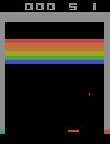
The following image shows a single frame took out from Atari game BreakOut. From this image, the agent is able to capture information about the location of the ball, the location of the board, etc. But several important information is not shown. If you play as the agent, this image is shown to you, what action you will choose? Feel something is missing? Is the ball going right or left? Is the ball going up or down?
Generated Using openAI Gym
The following images are two continuous frames took out from the game BreakOut. From these two images that agent is able to capture the information on the direction of the ball and also the speed of the ball. A lot of people tends to forget this since processing recent memories during playing a game is like a nature to us but not to an reinforcement agent.


Generated Using openAI Gym
Agent Play in CartPole environment
The main environment for agent to learn and tested is CartPole environment. This environment is consist of two movable parts. One is the cart which is controlled by the agent, has two possible action every state which is moving left or right. The other one is pole. This environment simulate the effect of gravity on pole which makes it fall to left or right due to its orientation with the horizon. For this environment to be considered as solved, the average episodes that the agent able to get in 100 games is over 195. Following graph is a visual representation of the environment. The blue rectangle represents the pole. The black box is the cart. The black line is the horizon.

First, let's create an environment
$env = RLEnvironmentCreate["WLCartPole"]
Then, initialize a network for this environment and a generator
policyNet =
  NetInitialize@
   NetChain[{LinearLayer[128], Tanh, LinearLayer[128], Tanh,
     LinearLayer[2]}, "Input" -> 8,
    "Output" -> NetDecoder[{"Class", {0, 1}}]];
generator := creatGenerator[$env, 20, 10000, False, 0.98, 1000, 0.95, False]
The generator function plays the game and generates input-output pairs to train the network. Inside the generator, it initialize the replay buffer which is processed, reward list is used to record the performance, best is to record the peak performance.
If[#AbsoluteBatch == 0,
         processed = <|"action"->{},"observation"->{},"next"->{},"reward"->{}|>;
         $rewardList = {};
         $env=env;
         best = 0;
       ];
Then the environment data are being generated from game function and being preprocessed. At the start of training, the generator will produce more data to fill the replay buffer.
If[#AbsoluteBatch == 0,
         experience = preprocess[game[start,maxEp,#Net, render, Power[randomDiscount,#AbsoluteBatch], $env], nor]
         ,
         experience = preprocess[game[1,maxEp,#Net, render, Power[randomDiscount,#AbsoluteBatch],$env], nor]
       ];
The game function is below, it is joining current observation and next observation as the input to the network.
game[ep_Integer,st_Integer,net_NetChain,render_, rand_, $env_, end_:Function[False]]:= Module[{
       states, list,next,observation, punish,choiceSpace,
       state,ob,ac,re,action
    },
    choiceSpace = NetExtract[net,"Output"][["Labels"]];
    states = <|"observation"->{},"action"->{},"reward"->{},"next"->{}|>;
    Do[
       state["Observation"] = RLEnvironmentReset[$env]; (* reset every episode *)
       ob = {};
       ac = {};
       re = {};
       next = {};
       Do[
         observation = {};
         observation = Join[observation,state["Observation"]];

         If[ob=={},
          observation = Join[observation,state["Observation"]]
          ,
          observation = Join[observation, Last[ob][[;;Length[state["Observation"]]]]]
         ];

           action = If[RandomReal[]<=Max[rand,0.1],
               RandomChoice[choiceSpace]
               ,
               net[observation]
            ];

         (*Print[action];*)
         AppendTo[ob, observation];
         AppendTo[ac, action];

         state = RLEnvironmentStep[$env, action, render];

         If[Or[state["Done"], end[state]],
          punish = - Max[Values[net[observation,"Probabilities"]]] - 1;
          AppendTo[re, punish];
          AppendTo[next, observation];
          Break[]
          ,
          AppendTo[re, state["Reward"]];
          observation = state["Observation"];
          observation = Join[observation, ob[[-1]][[;;Length[state["Observation"]]]]];
          AppendTo[next, observation];
         ]?

         ,
         {step, st}];
       AppendTo[states["observation"], ob];
       AppendTo[states["action"], ac];
       AppendTo[states["reward"], re];
       AppendTo[states["next"], next];
       ,
       {episode,ep}
    ];
    (* close the $environment when done *)
    states
]
Preprocess function flatten the input and has an option on if normalizing the observation
preprocess[x_, nor_:False] := Module[{result},(
    result = <||>;
    result["action"] = Flatten[x["action"]];
    If[nor,
       result["observation"] = N[Normalize/@Flatten[x["observation"],1]];
       result["next"] = N[Normalize/@Flatten[x["next"],1]];
       ,
       result["observation"] = Flatten[x["observation"],1];
       result["next"] = Flatten[x["next"],1];
    ];
    result["reward"] = Flatten[x["reward"]];
    result
)]
Let's continue with generator, after getting the data from the game, generator measures the performance and records it.
       NotebookDelete[temp];
       reward = Length[experience["action"]];
       AppendTo[$rewardList,reward];
       temp=PrintTemporary[reward];
Records the net with best performance
If[reward>best,best = reward;bestNet = #Net];
Add these experience to the replay buffer
                    AppendTo[processed["action"],#]&/@experience["action"];
         AppendTo[processed["observation"],#]&/@experience["observation"];
         AppendTo[processed["next"],#]&/@experience["next"];
         AppendTo[processed["reward"],#]&/@experience["reward"];
Make sure the total size of replay buffer does not exceed the limit len = Length[processed["action"]] - replaySize; If[len > 0, processed["action"] = processed["action"][[len;;]]; processed["observation"] = processed["observation"][[len;;]]; processed["next"] = processed["next"][[len;;]]; processed["reward"] = processed["reward"][[len;;]]; ]; Add input of the network to the result
pos = RandomInteger[{1,Length[processed["action"]]},#BatchSize];
result = <||>;
result["Input"] = processed["observation"][[pos]];
Calculates the out put based on the next state and reward and add to the result
predictionsOfCurrentObservation = Values[#Net[processed["observation"][[pos]],"Probabilities"]];
rewardsOfAction  = processed["reward"][[pos]];
maxPredictionsOfNextObservation = gamma*Max[Values[#]]&/@#Net[processed["next"][[pos]],"Probabilities"];
temp = rewardsOfAction + maxPredictionsOfNextObservation;
MapIndexed[
    (predictionsOfCurrentObservation[[First@#2,(#1+1)]]=temp[[First@#2]])&,(processed["action"][[pos]]-First[NetExtract[net,"Output"][["Labels"]]])
];
result["Output"] = out;
result
In the end, we can start training
trained =
 NetTrain[policyNet, generator,
  LossFunction -> MeanSquaredLossLayer[], BatchSize -> 32,
  MaxTrainingRounds -> 2000]
Performance of the agent
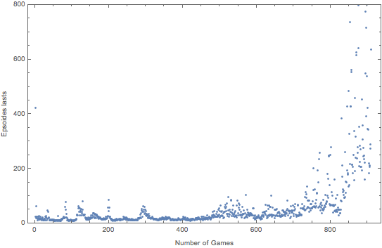
The graph above show the performance of the agent in 1000 games in cart pole environment. The agent starts with random play which has a low number of episodes lasted. The performance stay low till 800 games. But after 800 games, the performance starts to increase exponentially. In the end of the training, the performance jumps from 3k to 10k which is the maximal number of episode per game in 4 games. This proves that although the Q function is hard to converge, but when it converges, the performance is very well.
Future Directions
The current agent uses the classical DQN as its major structure. Other techniques like Noisy Net, DDQN, Prioritized Reply, etc can help the Q function to converge in a shorter time. Other algorithms like Rainbow Algorithm which is based on Q learning will be the next step of this project.
code can be found on github link