INTRODUCTION

Morphing or "metamorphosis" is a technique used to generate a sequence of images that smoothly transform a source image into a target image. This technique is often used to create special effects for motion pictures or television commercials. A conventional method used for generating smooth transformations is by first warping the source and the target images so that the features on both images are aligned to each other and then cross-dissolving the colors of the warped images.

There are two main hurdles to overcome in this approach: -

1. Extracting features from the source and the target images and establishing a correspondence between them: this concerns the amount of effort required by the user to specify the correspondence between the source and the target images.
2. Interpolating image key points to generate features for the intermediate image: this becomes complicated especially when rotation is involved.

Here we attempt to find a solution to the feature interpolation problem. The goal of this project is to create a morph between two images using semantic segmentation and geometric interpolation.

METHODS

We approached this problem by breaking it into three steps: -

Segmentation

The first step was to create a segment of the region of interest. This helps isolate feature detection only to the concerned object without picking up the background noise. After unsuccessfully segmenting images using Wolfram Language's image processing features, we turned our attention towards semantic segmentation. For this, we implemented the Ademxapp Model A1 which is a convolution neural network model that performs semantic pixel-wise segmentation. We selected this model because of its high IoU accuracy on the PASCAL VOC2012, a rich classification and segmentation dataset.

NetEvaluate[img_, device_: "CPU"] := Block[
  {net, resized, encData, dec, mean, var, prob},
  net = NetModel[
    "Ademxapp Model A1 Trained on PASCAL VOC2012 and MS-COCO Data"];
  resized = ImageResize[img, {504}];
  encData = Normal@NetExtract[net, "Input"];
  dec = NetExtract[net, "Output"];
  {mean, var} = Lookup[encData, {"MeanImage", "VarianceImage"}];
  prob = NetReplacePart[net,
     {"Input" -> 
       NetEncoder[{"Image", ImageDimensions@resized, 
         "MeanImage" -> mean, "VarianceImage" -> var}], 
      "Output" -> Automatic}
     ][resized, TargetDevice -> device];
  prob = ArrayResample[prob, 
    Append[Reverse@ImageDimensions@img, 21]];
  dec[prob]
]


$netModel := NetModel["Ademxapp Model A1 Trained on PASCAL VOC2012 and MS-COCO Data"];
SegmentImage[img_] := Block[
    {labels, objectshape},
    labels = {"background", "airplane", "bicycle", "bird", "boat", 
       "bottle", "bus", "car", "cat", "chair", "cow", "table", "dog", 
       "horse", "motorcycle", "person", "plant", "sheep", "sofa", "train", 
       "television"};
    objectshape = Binarize[Colorize[NetEvaluate[img]]]
]

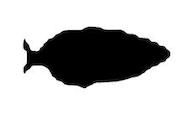
The trained network performed fairly well even on low contrast images.

In[ $\cdot$]:= SegmentImage /@ {,}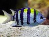

Out[ $\cdot$]:= {,}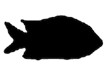

We then performed image processing on the obtained mask to get the desired object.

Mapping

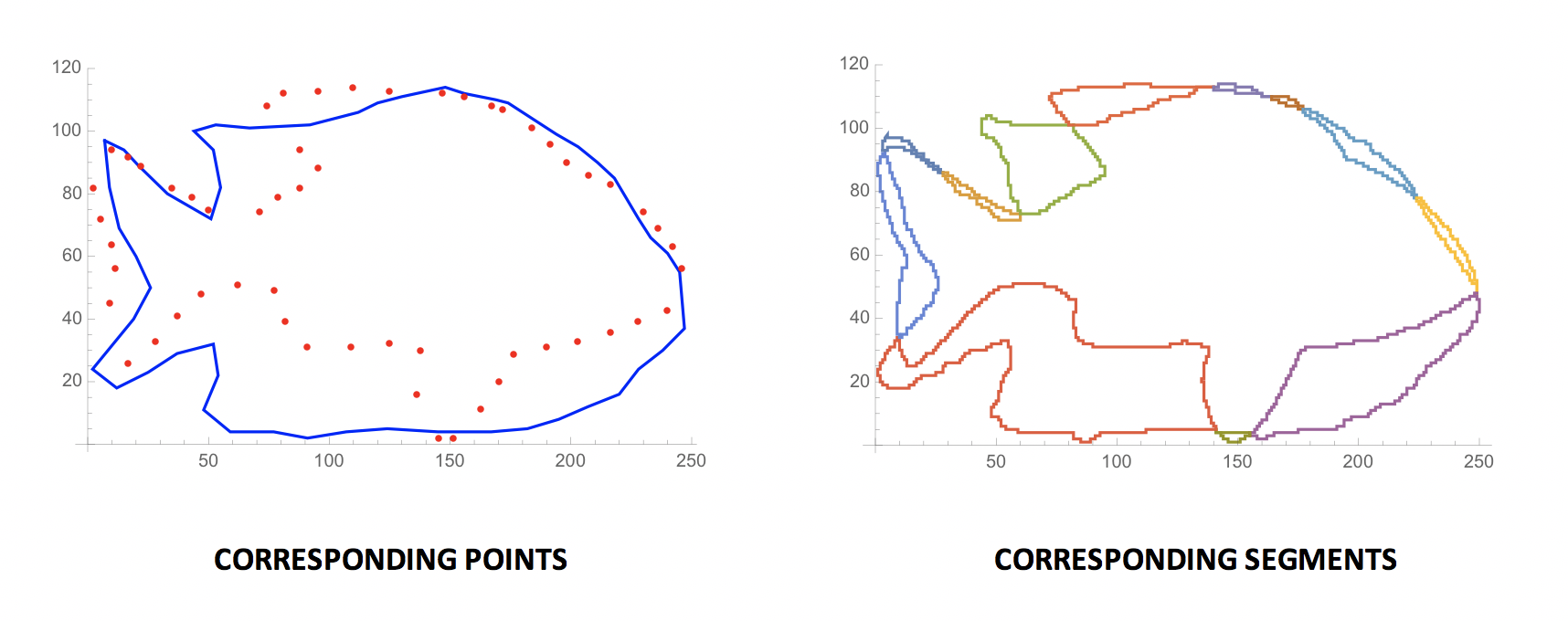
The second step was to find a one-to-one mapping between the points on the perimeter of the two objects. This would later be useful in describing the required spatial transformation. To simplify the problem, we made two convenient albeit restrictive assumptions: the input images must be aligned and partially overlapping. With these assumptions, we devised an algorithm to find a segment-to-segment correspondence. The algorithm first finds all the intersection points between the object perimeters. Then, it radially cleans any intersection clusters within 2% of the image dimensions. Next, it finds an ordered list of points for each object perimeter and categorizes them into segments. Finally, it resamples these points so they are equal and uniformly distributed. We can then pair points at corresponding indices to generate a list of transformation vectors.

Pseudocode of the algorithm

Input: Two aligned and partially overlapping

Algorithm:

1. Find intersection points
2. Remove intersection clusters
3. Find ordered list of points around the object perimeter
4. Categorize boundary points into segments
5. Resample so that the number of points are equal and uniformly distributed

Output: List of transformation vectors

TourPoints::usage = "TourPoints[points, firstintersection] returns a sorted List of points starting from firstintersection.";

TourPoints[points_List, firstintersection_] := Block[
    {startpt, tour},
    startpt = Position[points, firstintersection][[1,1]];
    tour = FindShortestTour[points, startpt, startpt] // Last;
    points[[tour]]
]


SegmentPoints::usage = "SegmentPoints[tourpts, breakpts] returns a nested List of elements in tourpts that are present between each pair of consecutive breakpts.";

SegmentPoints[tourpts_List, breakpts_List] := Block[
    {positions, rotatedpos},
    positions = Sort[Position[tourpts, #]&/@breakpts];
    rotatedpos = Append[Drop[positions,1], {{All}}];
    MapThread[tourpts[[#1[[1,1]] ;; #2[[1,1]]]]&, {positions,rotatedpos}]
]


SelectPoints::usage = "SelectPoints[l, n] returns n equispaced elements from List l.";

SelectPoints[l_List, n_] := Block[
    {totake},
    totake = Round[Range[n]*(Length[l]/(n+1))];
    l[[totake]]
]

Interpolation

The final step of this project was to implement an interpolation function for the obtained list of transformation vectors. To achieve this we implemented a warping algorithm using Thin Plate Spline (TPS), an effective tool for modeling coordinate transformations. The main advantage of TPS over competing geostatistical techniques is that splines do not require prior approximation of spatial auto-covariance structure which can be difficult to estimate and validate. Unfortunately, the solution requires the inversion of a p×p matrix, where p is the number of points in the data set, thus making it impractical for large scale applications. To address this problem we adopted a technique for function approximation using radial basis functions (RBFs).

A radial basis interpolation function has the form $\begin{equation} y(x) = \sum _{i=1}^n w_i \phi \left(x-x_i\right)+a\cdot x+a_0 \end{equation}$. Here, $a_0$ and $a$ determine the linear part of the interpolation function, $w_i$ is the weight at basis $x_i$, and $\phi$ is a function that returns a vector norm of the vector $x-x_i$. In the case of a thin plate spline interpolation, the vector norm is given by the thin plate spline norm $\begin{equation} \phi(x) = x\cdot x \log \left(\sqrt{x\cdot x}\right) \end{equation}$.

Parameters $a$ and $w_i$ are estimated by solving the linear system $\begin{equation} \left(\begin{array}{cc} B-\lambda I & Q\\ Q^T & 0 \end{array}\right) \left(\begin{array}{c} w \\ a \end{array}\right) = \left(\begin{array}{c} y \\ 0 \end{array}\right) \end{equation}$, where $\begin{equation} B = (b_{ij}) = \phi \left(x-x_i\right) \end{equation}$, $\lambda$ is the smoothness parameter, and $\begin{equation} Q = \begin{pmatrix} 1 & x_{1,1} & x_{1,2} & \cdots & x_{1,d} \\ 1 & x_{2,1} & x_{2,2} & \cdots & x_{2,d} \\ \vdots & \vdots & \vdots & \ddots & \vdots \\ 1 & x_{n,1} & x_{n,2} & \cdots & x_{n,d} \\ \end{pmatrix} \end{equation}$, with $d$ being the number of dimensions and $n$ the number of basis points.

RadialBasisInterpolation::usage = "RadialBasisInterpolation[source, target, \[Lambda]] creates a compiled thin plate spline interpolation functions that maps the List of source points onto the List of target points. \[Lambda] is a smoothness parameter.";

RadialBasisInterpolation[sources_List, targets_List, \[Lambda]_?NumberQ,(opts___)?OptionQ] := Module[
       {n, dim, Q, \[Phi], B, M, wa},
       {n, dim} = Dimensions[sources];
       Q = PadLeft[sources, {n, dim+1}, 1];
       \[Phi] = ThinPlateSplineNorm[2];
       B = Map[\[Phi], Outer[Subtract, sources, sources, 1], {2}];
       M = ArrayFlatten[{{B-\[Lambda] IdentityMatrix[n], Q}, {Transpose[Q], ConstantArray[0, {dim,dim}+1]}}];
       Off[LinearSolve::luc];
         wa = Map[LinearSolve[M, PadRight[#, n+dim+1]]&, Transpose[targets]];
       On[LinearSolve::luc];
       Compile[{{x, _Real, 1}}, #1+#2.x+#3.Map[#4, Transpose[x-#5]]]& [wa[[All,-(dim+1)]], Take[wa,All,-dim], Take[wa,All,n], \[Phi], Transpose[sources]]
] /; Dimensions[sources] === Dimensions[targets]


ThinPlateSplineNorm::usage = "ThinPlateSplineNorm[n][v] returns the n-th thin plate spline norm of vector v.";

ThinPlateSplineNorm[1] = Sqrt[#.#]&;
ThinPlateSplineNorm[2] = (If[#>0, # Log[#]/2, 0]& [#.#])&;
ThinPlateSplineNorm[p_?OddQ] := (#.#)^(p/2)&;
ThinPlateSplineNorm[p_?EvenQ] := (If[#>0, #^(p/2) Log[#]/2, 0]& [#.#])&;

RESULTS AND CONCLUSION

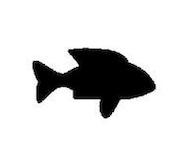
The proposed technique works only for objects that are aligned and partially overlap. It works best for images that have low density of intersection points. This is because the RBF interpolation used in the algorithm tears the 2D space for overlapping vectors. This method does not extract features from the images, but rather exploits the curvature of the splines. The quality of the results obtained is also guided by the accuracy of the segmentation algorithm.

In[ $\cdot$]:= MorphImage[,]

Out[ $\cdot$]:=

FUTURE WORK

Many different adaptations, tests, and experiments were left out due to lack of time. Some of the ideas that we would have liked to try during the development of this project are: -

1. Implement a shape interpolation scheme to produce results with a bounded amount of conformal distortion
2. Extract matching features for image alignment and local warping
3. Develop a morphing sequence from automatically generated sparse correspondence points

REFERENCES

• Wolfram Neural Net Repository
• H. Johan, Y. Koiso, T. Nishita, "Morphing using curves and shape interpolation techniques", Proceedings the Eighth Pacific Conference on Computer Graphics and Applications, pp. 348-454, 2000.

Attachments:

MorphImage.wl