Introduction

The purpose of this project is to compute statistical properties of craters on the moon from an image. The core of this project was a function called MorphologicalBinarize, which essentially creates a binarized version of the inputted image, decides upon an upper threshold for an image and replaces all values greater than that threshold with a 1.. The pictures of the surface of the moon that I acquired, from NASA, were birds-eye view pictures, so the craters would appear to be circular, and could be outlined to perform computations on. The computations that I did were returning the approximate number of craters in the image, in a range, a graphic showing the distribution of crater sizes, and another graphic showing the distribution of distances between craters.

Number of Craters From an Image

The first step was essentially experimentation with image processing functions, and finding circles. However, in order to return the number of craters, I first had to define another function for that specific purpose.

numberofcraters[randimg_Image] := 
 Module[{upperthresh, lowerbound, upperbound, lowisolimg, upisolimg}, 
  upperthresh = FindThreshold[randimg];
  lowisolimg = 
   EdgeDetect[MorphologicalBinarize[randimg, {0.31, upperthresh}]];
  upisolimg = 
   EdgeDetect[MorphologicalBinarize[randimg, {0.36, upperthresh}]];
  lowerbound = 
   Length[ComponentMeasurements[lowisolimg, "Area"][[All, 2]]];
  upperbound = 
   Length[ComponentMeasurements[upisolimg, "Area"][[All, 2]]];
  {lowerbound, upperbound}]

This function takes in an image as input, and essentially returns a range between which the number of craters in the picture is estimated to be. Note that it only will work for birds-eye views. MorphologicalBinarize takes in two arguments, an image and a range for which to binarize, which in this case is replace all values above the upper bound with a 1, and the upper bound of that range is FindThreshold of the image. ComponentMeasurements is used because it has the ability to find the area of each crater isolated by MorphologicalBinarize. ComponentMeasurements takes the property of a given image, which here will be "Area", and it computes this property for the components of the image which it isolates with a given matrix. It will return a long list of areas for each crater. Then Length is applied to the list to get the number of craters. In order to create an lower and upper bound, two different arguments were used in MorphologicalBinarize, and then Length was applied.

Distribution of Crater Sizes

Now that the number of craters has been defined, I was able to define a function that would actually return the distributions.

CraterSizeDistr2[img_Image, checkbox_] := 
 Module[{areaofcraterslist, avgcratersize, stdevcratersize, hist1, 
   hist2, dataset1, numofcraters, upperthresh2, min2cratersize, 
   max2cratersize, mostcommonelement, highlightedimg, realdistr2, 
   listofallcenters, distanceallcenters, hist3}, 
  upperthresh2 = FindThreshold[img];
  areaofcraterslist = 
   ComponentMeasurements[
     EdgeDetect[MorphologicalBinarize[img, {0.28, upperthresh2}]], 
     "Area"][[All, 2]];
  avgcratersize = Mean[areaofcraterslist];
  stdevcratersize = StandardDeviation[areaofcraterslist];
  min2cratersize = Min[areaofcraterslist];
  max2cratersize = Max[areaofcraterslist];
  mostcommonelement = Commonest[areaofcraterslist];
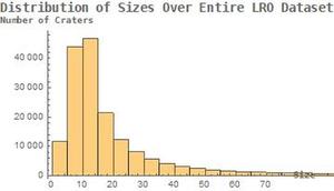
  realdistr2 = ImageResize[Image, 700];
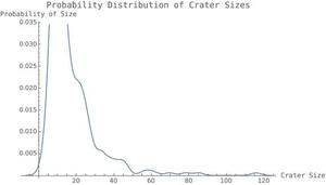
  hist2 = 
   SmoothHistogram[areaofcraterslist, 
    PlotLabel -> 
     Style["Probability Distribution of Crater Sizes", FontSize -> 14,
       FontFamily -> "Bitstream Vera Sans Mono"], 
    AxesLabel -> {Style["Crater Size", FontSize -> 11, 
       FontFamily -> "Bitstream Vera Sans Mono"], 
      Style["Probability of Size", FontSize -> 11, 
       FontFamily -> "Bitstream Vera Sans Mono"]}, ImageSize -> Large];
  dataset1 = 
   Dataset[{<|"Mean" -> avgcratersize, 
      "Standard Deviation" -> stdevcratersize|>}];
  highlightedimg = 
   HighlightImage[img, EdgeDetect[MorphologicalBinarize[img]]];
  listofallcenters = 
   Subsets[ComponentMeasurements[
      EdgeDetect[MorphologicalBinarize[img]], "BoundingDiskCenter"][[
     All, 2]], 2];
  distanceallcenters = Map[distancelistlists, listofallcenters];
  hist3 = 
   Histogram[distanceallcenters, 
    PlotLabel -> 
     Style["Distribution of Distances Between Craters", 
      FontFamily -> "Bitstream Vera Sans Mono", FontSize -> 12], 
    AxesLabel -> {Style["Distance", 
       FontFamily -> "Bitstream Vera Sans Mono", FontSize -> 8], 
      Style["Number of Craters with that Distance", 
       FontFamily -> "Bitstream Vera Sans Mono", FontSize -> 8], 
      ImageSize -> Large, 
      FrameTicks -> {{Style[Automatic, 
          FontFamily -> "Bitstream Vera Sans Mono", FontSize -> 1], 
         None}, {Style[Automatic, 
          FontFamily -> "Bitstream Vera Sans Mono", FontSize -> 1], 
         None}}}];
  Switch[checkbox, True, cratercount = 0.5*numberofcraters2[img], 
   False, cratercount = numberofcraters[img]];
  Grid[{{Style[
      "The Number of Craters is Estimated to be between " <> 
       ToString[cratercount[[1]]] <> " and " <> 
       ToString[cratercount[[2]]], FontSize -> 20, 
      FontFamily -> "Bitstream Vera Sans Mono"], 
     SpanFromLeft}, {hist2, SpanFromLeft}, {realdistr2, 
     ImageResize[hist3, 800]}, {ImageResize[highlightedimg, 500], 
     SpanFromLeft}, {Grid[{{"Size Distribution", 
        SpanFromLeft}, {"Mean", avgcratersize}, {"Standard Deviation",
         stdevcratersize}, {"Smallest Crater Size", 
        min2cratersize}, {"Largest Crater Size", 
        max2cratersize}, {"Most Common Crater Size", 
        mostcommonelement}}, Frame -> All], SpanFromLeft}}]]

After I had all my variables, which aided in the computations and were used to hold values until they were ready for the display, I simply compiled everything into a grid, which lets me arrange everything however I want, whether in a column, side-by-side, etc. Some sample graphics are shown below. Something that is worth noting is the Switch with the checkbox inside. Many thanks to Andrea for helping me create this, and for a lot of help with the microsite. When MorphologicalBinarize was called on darker images, it tended to group everything together and provide very inaccurate results. For example, in an image that was expected to have around 200 craters, it predicted closer to 500. The algorithm applies MorphologicalBinarize, which looks for the outline of the crater and identifies it as a crater. However, with shadows, it treats everything as an outline, therefore providing more craters than there actually are. In order to solve this problem, I defined a second number-of-craters function, numberofcrater2, which was the same as the original, but has slightly different parameters in the MorphologicalBinarize function, to provide smaller estimates for the number of craters. This could be done by creating a "darkness scale" of some sorts, and implementing this into Mathematica so before applying the function to the given image, it could first analyze the image for darkness and decide on correct parameters. It could also zoom in, and analyze the image in smaller chunks and then piece everything together.. Also, the line with ImageResize[Image,700], resized an image of the distribution of crater sizes over the entire dataset of moon pictures from NASA, which can be compared to each individual image. This was the main part of the project, as it was my initial goal. However, this did not take very long to do, and afterwards, I had many directions to continue in.

Highlighting the Number of Craters Detected By My Algorithm

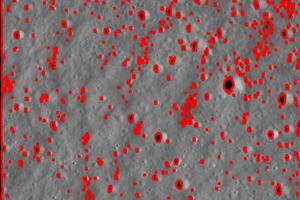
To provide an image of how many craters my algorithm actually accounted for, I used the HighlightImage function:

highlightedimg = 
 HighlightImage[img, EdgeDetect[MorphologicalBinarize[img]]]

The input, img, is the same as the input of the CraterSizeDistr2 because the highlighted img code is within that function.

Distribution of Distances Between Craters

The second extension was upon another distribution. However, instead of having something to do with size, this instead mapped all the distances between any two craters to a histogram. The process for doing this was essentially the same as for the distribution of areas; ComponentMeasurement very conveniently has an argument that includes the center coordinates of each crater, so I was able to utilize this, take all subsets of the list, apply EuclideanDistance, which simply finds the distance between 2 vectors, and then creates a histogram. However, there was a slight issue. Because the EuclideanDistance takes two arguments, which are lists, and the ComponentMeasurements returns a list of lists, which each contain two lists. So, I had to define a function to apply EuclideanDistance to a list containing two lists each, and then map that to the entire list.

distancelistlists[lst_List] := 
 Module[{firstlist, secondlist}, firstlist = lst[[1]];
  secondlist = lst[[2]];
  EuclideanDistance[firstlist, secondlist]]

distanceallcenters = Map[distancelistlists, listofallcenters];

hist3 = Histogram[distanceallcenters, 
   PlotLabel -> 
    Style["Distribution of Distances Between Craters", 
     FontFamily -> "Bitstream Vera Sans Mono", FontSize -> 12], 
   AxesLabel -> {Style["Distance", 
      FontFamily -> "Bitstream Vera Sans Mono", FontSize -> 8], 
     Style["Number of Craters with that Distance", 
      FontFamily -> "Bitstream Vera Sans Mono", FontSize -> 8], 
     ImageSize -> Large, 
     FrameTicks -> {{Style[Automatic, 
         FontFamily -> "Bitstream Vera Sans Mono", FontSize -> 1], 
        None}, {Style[Automatic, 
         FontFamily -> "Bitstream Vera Sans Mono", FontSize -> 1], 
        None}}}];

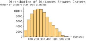
The distancelistlists function was what took the EuclideanDistance, the distanceallcenters was what mapped the function to the entire list, and the hist3 was just recording all the data in a histogram. This particular part of the code was sort of a side project; that is, it wasn't in the initial project design, I just decided that I had time, and implementing it would be something that I thought would be interesting.

Cloud Deployment

The last step was the actual deployment to the cloud, in the form of a microsite, which I also got a ton of help on from Andrea. The basic deployment wasn't too hard; I simply coded it so that the microsite accepted an input, in the form of an image and an option to select if there were shadows, which was where the numberofcraters2 came in. However, the complications arose when I realized that the microsite looked completely blank, as it wasn't styled in any way, shape or form. This meant I had to add color, labels, and things as such to essentially make the site look nicer. There was also some bit of styling that needed to be done for the graphics as well.

form5 = FormFunction[{"Img" -> <|"Interpreter" -> "Image", 
      "Label" -> "Insert an Image of the Moon"|>, 
    "Checkbox" -> <|"Interpreter" -> {"Yes" -> True, "No" -> False}, 
      "Label" -> "Are there shadows?"|>}, r, 
   AppearanceRules -> <|
     "Title" -> "The Distribution of Craters on the Moon", 
     "Description" -> 
      "This site will give you an estimate for the number of craters \
in the image you input, and also give you a distribution of the \
sizes, along with some statistics.", "ItemLayout" -> "Vertical", 
     "PageTheme" -> "Blue", 
     "SubmitLabel" -> "Tell Me Something About the Image!"|>];
r[assoc_] := CraterSizeDistr2[assoc["Img"], assoc["Checkbox"]];
CloudDeploy[form5, "Distribution of Craters on the Moon", 
 Permissions -> "Public"]

The r function referenced in the first line of code is a function that takes in the associations, indicated by the <||>, and returns the CraterSizeDistr2 evaluated with that assoc. This essentially is just telling the microsite to evaluate the function at the image input from the user, and the checkbox is to indicate whether to use numberofcraters or numberofcraters2, so as to use the correct parameters for MorphologicalBinarize.

Conclusion

The functions that I implemented take an image of the moon, (assuming a bird's-eye view ) and return the number of craters estimated to be in the image, in a range, a graphic of the distribution of crater sizes over the particular picture and over the entire dataset, a distribution of crater distances, a highlighted image highlighting the craters detected by my algorithm, and some statistics about the inputted image, such as Mean, Standard Deviation, etc. I would like to thank Andrea and Rob for all the help they gave me in completing my project, along with the other mentors. I would also like to thank Dr. Wolfram and the Wolfram High School Summer Camp for the opportunity to become engaged in such an adventure, and one that will remain with me for years to come.