Abstract
This project aims to develop a machine learning application to identify the sentiments in a music clip. The data set I used consists of one hundred 45-second clips from the Database for Emotional Analysis of Music and an additional 103 gathered by myself. I manually labeled all 203 clips and used them as training data for my program. This program works best with classical-style music, which is the main component of my data set, but also works with other genres to an reasonable extent.
Introduction
One of the most important functions of music is to affect emotion, but the experience of emotion is ambiguous and subjective to individual. The same music may induce a diverse range of feelings in people as a result of different context, personality, or culture. Many musical features, however, usually lead to the same effect on the human brain. For example, louder music correlates more with excitement or anger, while softer music corresponds to tenderness. This consistency makes it possible to train a supervised machine learning program based on musical features.
Background
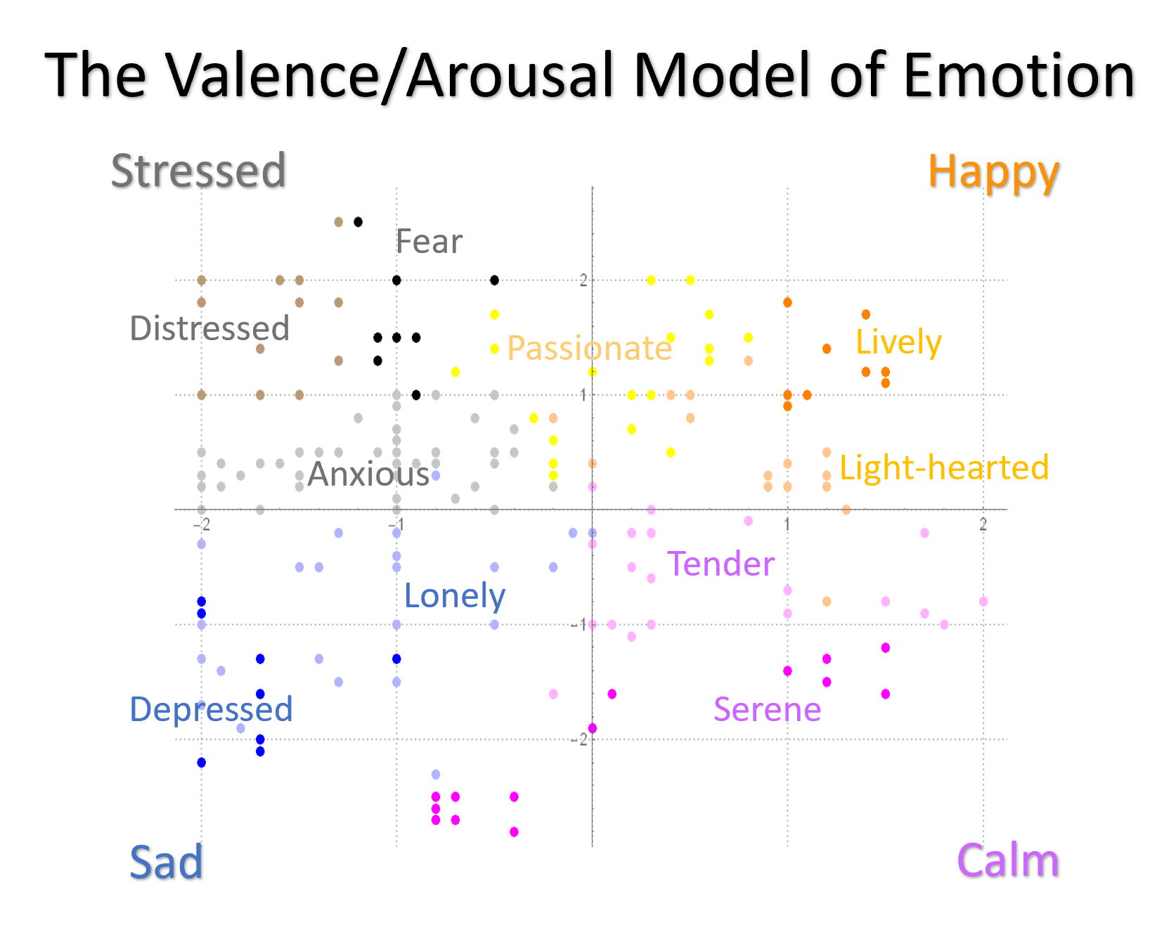
This project is based on James Russell's circumplex model, in which a two-dimensional emotion space is constructed from the x-axis of valence level and y-axis of arousal level, as shown above in the picture. Specifically, valence is a measurement of an emotion's pleasantness, whereas arousal is a measurement of an emotion's intensity. Russell's model provides a metric on which different sentiments can be compared and contrasted, creating four main categories of emotion: Happy (high valence, high arousal), Stressed (low valence, high arousal), Sad (low valence, low arousal), and Calm (high valence, low arousal). Within these main categories there are various sub-categories, labeled on the graph above. Notably, "passionate" is a sub-category that does not belong to any main category due to its ambiguous valence value.
Program Structure
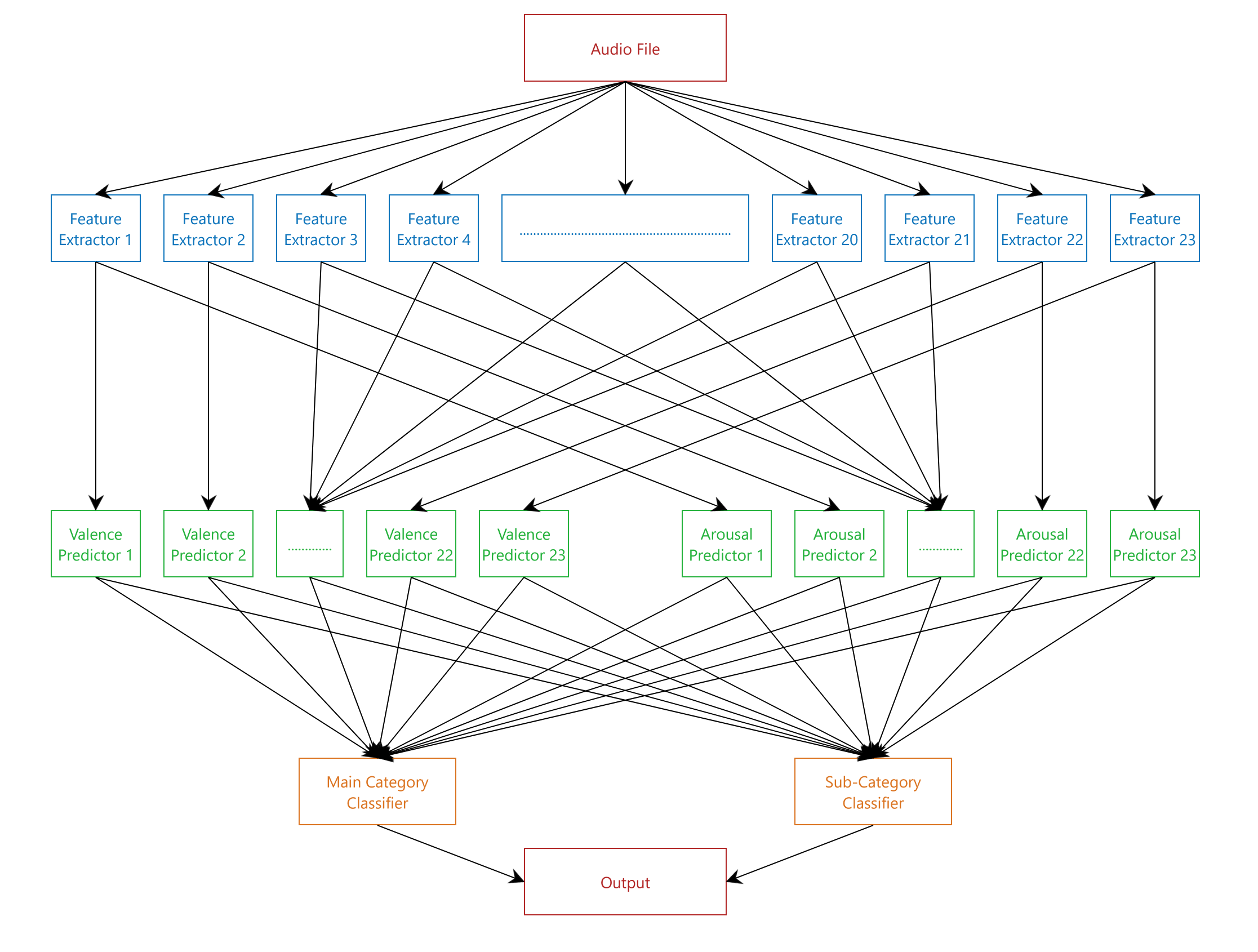
The program contains a three-layer structure. The first layer is responsible for extracting musical features, the second for generating a list of numerical predictions based on different features, and the third for predicting and displaying the most probable emotion descriptors based on the second layer's output.

First Layer
The first layer consists of 23 feature extractors that generate numerical sequence based on different features:
(*A list of feature extractors*)
feMin[audio_] := Normal[AudioLocalMeasurements[audio, "Min", List]]
feMax[audio_] := Normal[AudioLocalMeasurements[audio, "Max", List]]
feMean[audio_] := Normal[AudioLocalMeasurements[audio, "Mean", List]]
feMedian[audio_] := Normal[AudioLocalMeasurements[audio, "Median", List]]
fePower[audio_] := Normal[AudioLocalMeasurements[audio, "Power", List]]
feRMSA[audio_] := Normal[AudioLocalMeasurements[audio, "RMSAmplitude", List]]
feLoud[audio_] := Normal[AudioLocalMeasurements[audio, "Loudness", List]]
feCrest[audio_] := Normal[AudioLocalMeasurements[audio, "CrestFactor", List]]
feEntropy[audio_] := Normal[AudioLocalMeasurements[audio, "Entropy", List]]
fePeak[audio_] := Normal[AudioLocalMeasurements[audio, "PeakToAveragePowerRatio", List]]
feTCent[audio_] := Normal[AudioLocalMeasurements[audio, "TemporalCentroid", List]]
feZeroR[audio_] := Normal[AudioLocalMeasurements[audio, "ZeroCrossingRate", List]]
feForm[audio_] := Normal[AudioLocalMeasurements[audio, "Formants", List]]
feHighFC[audio_] := Normal[AudioLocalMeasurements[audio, "HighFrequencyContent", List]]
feMFCC[audio_] := Normal[AudioLocalMeasurements[audio, "MFCC", List]]
feSCent[audio_] := Normal[AudioLocalMeasurements[audio, "SpectralCentroid", List]]
feSCrest[audio_] := Normal[AudioLocalMeasurements[audio, "SpectralCrest", List]]
feSFlat[audio_] := Normal[AudioLocalMeasurements[audio, "SpectralFlatness", List]]
feSKurt[audio_] := Normal[AudioLocalMeasurements[audio, "SpectralKurtosis", List]]
feSRoll[audio_] := Normal[AudioLocalMeasurements[audio, "SpectralRollOff", List]]
feSSkew[audio_] := Normal[AudioLocalMeasurements[audio, "SpectralSkewness", List]]
feSSlope[audio_] :=  Normal[AudioLocalMeasurements[audio, "SpectralSlope", List]]
feSSpread[audio_] := Normal[AudioLocalMeasurements[audio, "SpectralSpread", List]]
feNovelty[audio_] := Normal[AudioLocalMeasurements[audio, "Novelty", List]]
Second Layer
Using data generated from the first layer, the valence and arousal predictors of the second layer provide 46 predictions for the audio input, based on its different features.
(*RMSAmplitude*)
(*Feature extractor*) feRMSA[audio_] := Normal[AudioLocalMeasurements[audio, "RMSAmplitude", List]]
dataRMSA = Table[First[takeLast[feRMSA[First[Take[musicFiles, {n}]]]]], {n, Length[musicFiles]}];
(*Generating predictor*) pArousalRMSA = Predict[dataRMSA -> arousalValueC]

Third Layer
The two parts of the third layer, main category classifier and sub-category classifier, each utilize the tensors generated in the second layer to make a prediction within their realm of emotion. The output consists of two parts, a main category emotion and a sub-category emotion.
(*Main*) emotionClassify1 = Classify[classifyMaterial -> emotionList1, PerformanceGoal -> "Quality"]
(*Sub*) emotionClassify2 = Classify[classifyMaterial -> emotionList2, PerformanceGoal -> "Quality"]

Output
If the program receives an input that is longer than 45 second, it will automatically clip the audio file into 45 second segments and return the result for each. If the last segment is less than 45 seconds, the program would still work fine on it, though with reduced accuracy. The display for each clip includes a main-category and a sub-category descriptor, with each of their associated probability also printed.
Sample testing: Debussy's Clair de Lune

Conclusion
The program gives very reasonable result for most music in the classical style. However, the program have three shortcomings that I plan to fix in later versions of the this program. Firstly, the program may give contradictory result (ex. happy and depressed) if the sentiment dramatically changes in the middle of a 45 second segment, perhaps reflecting the music's changing emotional composition. The current 45 second clipping window is rather long and thus prone to capture contradicting emotions. In the next version of this program, the window will probably be shortened to 30 or 20 seconds to reduce prediction uncertainty. Secondly, the program's processing speed has a lot of room of improvement. It currently takes about one and half minutes to compute an one minute audio file. In future versions I will remove relative ineffective feature extractors to speed things up. Lastly, the data used in creating this application is solely from myself, and therefore it is prone to my human biases. I plan to expand the data set with more people's input and more genres of music.
I have attached the application to this post so that everyone can try out the program.
Acknowledgement
I sincerely thank my mentor, Professor Rob Morris, for providing invaluable guidance to help me carry out the project. I also want to thank Rick Hennigan for giving me crucial support with my code.
 Attachments: