MODERATOR NOTE: a submission to computations art contest, see more: https://wolfr.am/CompArt-22
As was illustrated in the latest Wolfram Insider, "shape-shifting" and ambiguous views of space curves can be derived from the intersection of perpendicular cylinders.
My recent Wolfram Community contribution More on Intersecting Cylinders and "Ambiguous Rings" [1], gives the conditions to obtain fully closed intersections curves between the cylinders. A "tight fit" between the cross section of the polygonal cylinder and the longitudinal cross section (two parallel lines) of the circular cylinder.
This requires the radius of the circular cylinder and the offset between the cylinders adapted to the axial rotation of the polygonal cylinder. For regular polygons, this tight fit can easily be computed with some elementary analytical geometry. These are the tight fit conditions for a triangular cross section and an animation to verify:
fittedRadius3[t_] :=
 1/2 (Max[-Cos[1/6 (\[Pi] - 6 t)], Cos[\[Pi]/6 + t], Sin[t]] -
    Min[-Cos[1/6 (\[Pi] - 6 t)], Cos[\[Pi]/6 + t], Sin[t]])
fittedOffset3[t_] :=
 1/2 (Max[-Cos[1/6 (\[Pi] - 6 t)], Cos[\[Pi]/6 + t], Sin[t]] +
    Min[-Cos[1/6 (\[Pi] - 6 t)], Cos[\[Pi]/6 + t], Sin[t]])
Animate[ParametricPlot[
  1/2 Sec[2/
     3 ArcTan[Cot[(3 (\[Theta] - \[Theta]0))/2]]] {Cos[\[Theta]],
    Sin[\[Theta]]}, {\[Theta], 0, 2 \[Pi]},
  PlotStyle -> Directive[AbsoluteThickness[2], Blue],
  PlotRange -> 1.25, Background -> Black, ImageSize -> Small,
  TicksStyle -> 6,
  Prolog -> {{AbsoluteThickness[1], Dotted, Circle[]}, Red,
    AbsoluteThickness[2],
    Line[{{{-5,
        fittedRadius3[\[Theta]0] + fittedOffset3[\[Theta]0]}, {5,
        fittedRadius3[\[Theta]0] +
         fittedOffset3[\[Theta]0]}}, {{-5, -fittedRadius3[\[Theta]0 + \
\[Pi]] - fittedOffset3[\[Theta]0 + \[Pi]]}, {5, -fittedRadius3[\
\[Theta]0 + \[Pi]] - fittedOffset3[\[Theta]0 + \[Pi]]}}}], Red,
    AbsolutePointSize[5], Point[{0, fittedOffset3[\[Theta]0]}], Black,
     Point[{0, 0}]}], {\[Theta]0, 0, 2 \[Pi]},
 TrackedSymbols :> Manipulate]
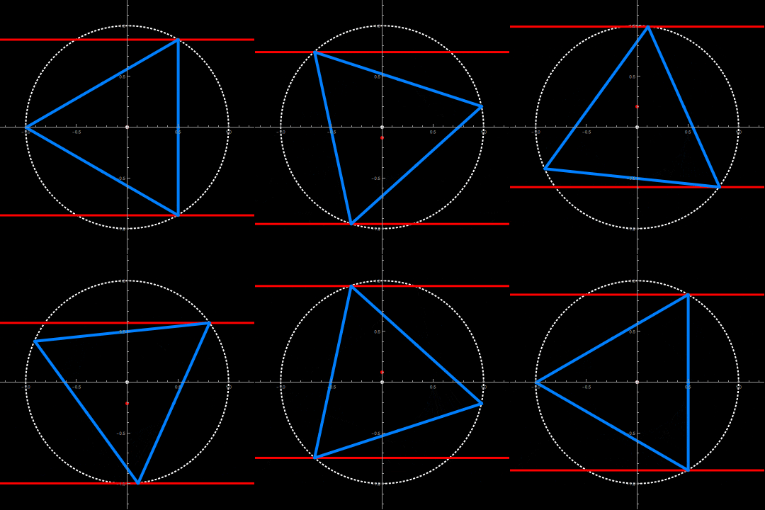
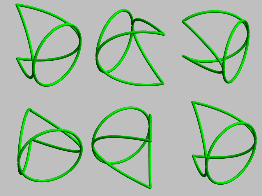
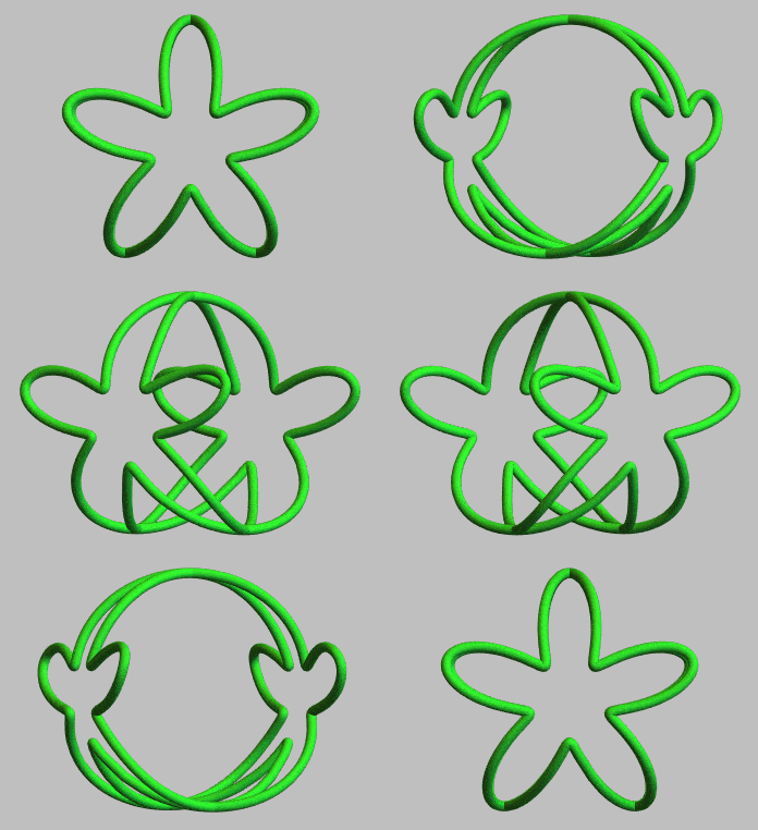
Entering this tight fit radius and -offset into the polyRingsetCF function from [1], we can make an animation scrolling through all possible closed intersections of a triangular and a circular cylinder:
Animate[Module[{n = 3, \[Alpha] = 0. r, d},
  r = fittedRadius3[\[Theta]0];
  d = fittedOffset3[\[Theta]0];
  ParametricPlot3D[
   polyRingsetCF[t, r, \[Theta]0, d,
    n, \[Alpha]], {t, -\[Pi], \[Pi]},
   PlotStyle -> {{Green, Tube[.035]}}, PerformanceGoal -> "Quality",
   SphericalRegion -> True, PlotRange -> 6,
   Background -> Lighter[Gray, 0.5], ViewPoint -> .7 {3, -3, 3},
   ViewAngle -> 4 \[Degree], Boxed -> False, Axes -> False]],
 {\[Theta]0, 0, 2 \[Pi]}]
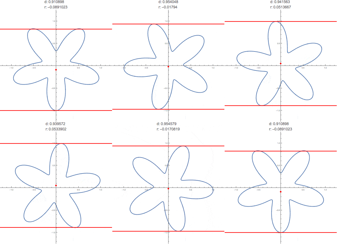
One can extend the idea of closed intersection curves showing shape-shifting to other than polygonal cylinders. An interesting case are intersections of rose-curve based cylinders (see my Wolfram Demonstration: "Ambiguous Rings Based on a Rose Curve" [2]. Here again, to a have tight fit of the cylinders, requires a radius and axial offset of the circular cylinder adapted to the axial rotation of the rose based cylinder.
Only in this case, it is not that simple to find an analytical solution. But we can find a numerical solution using the function FindMaxvalue to find the tangents for the parallel lines to the rose curve and build an interpolating function.
roseOf5[\[Theta]_, \[Theta]0_: 0](*parametric of a 5-petaled rose \
curve*):= {1/3 Cos[\[Theta]] (2 + Sin[\[Theta]0 + 5 \[Theta]]),
  1/3 Sin[\[Theta]] (2 + Sin[\[Theta]0 + 5 \[Theta]])}
tightFits =
  Table[{\[Theta]0,
    FindMaxValue[Last@roseOf5[\[Theta], \[Theta]0], \[Theta],
     PrecisionGoal -> 12,
     WorkingPrecision -> 16]}, {\[Theta]0, -\[Pi], \[Pi], \[Pi]/24}];
tightFitIF[\[Theta]0_] := Module[{f}, f = Interpolation[tightFits];
  Piecewise[{{f[Mod[\[Theta]0, 2 \[Pi]]],
     0 <= Mod[\[Theta]0, 2 \[Pi]] < \[Pi]}},
   f[Mod[\[Theta]0, 2 \[Pi]] - 2 \[Pi]]]]
fittedRadiusRose5[t_] := (tightFitIF[t] + tightFitIF[t + \[Pi]])/2;
fittedOffsetRose5[t_] := (tightFitIF[t] - tightFitIF[t + \[Pi]])/2;
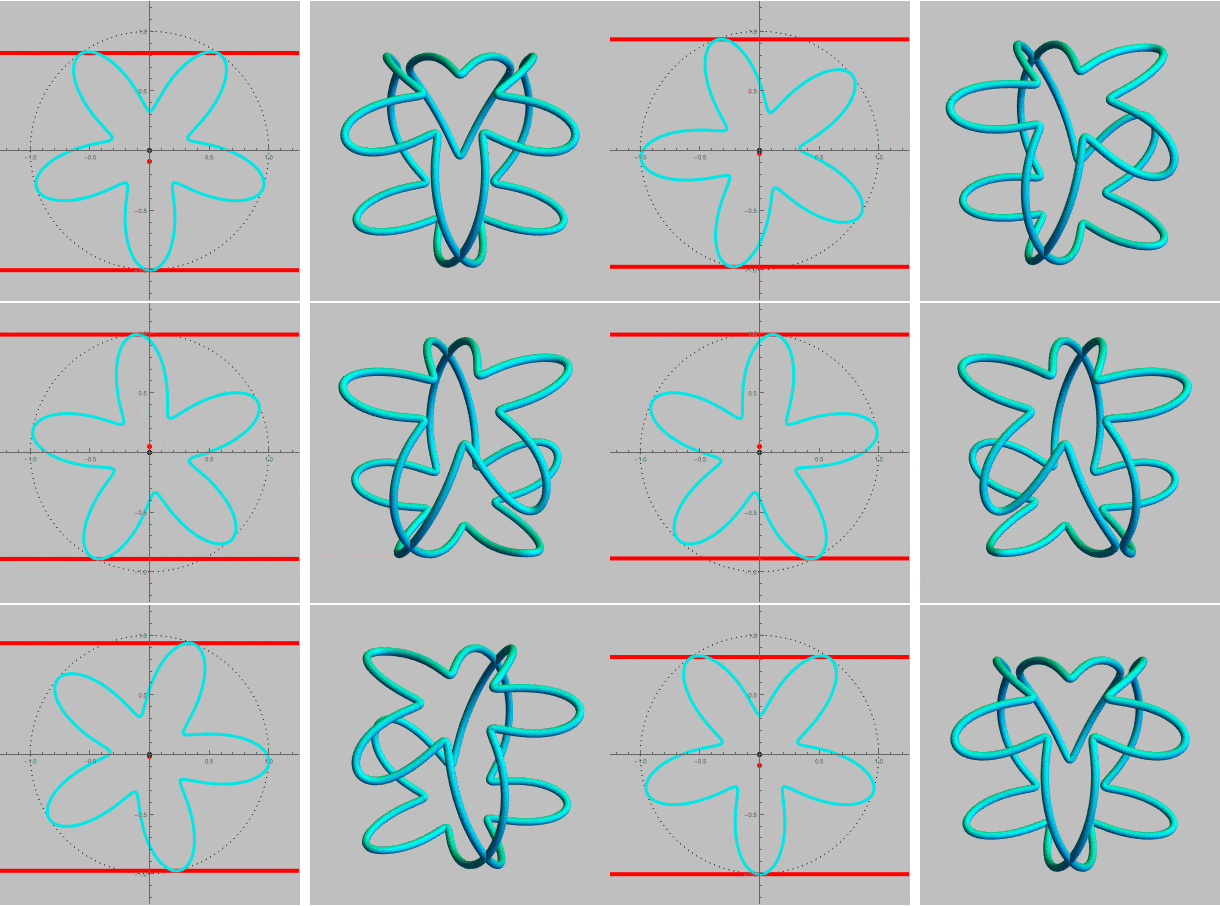
The tight fit can be demonstrated with an animation:
Animate[Quiet@
  ParametricPlot[roseOf5[\[Theta], \[Theta]0], {\[Theta], 0, 2 \[Pi]},
    PlotStyle -> Directive[AbsoluteThickness[4], Blue],
   PlotRange -> 1.25,
   Prolog -> {{Thick, Dotted, Circle[]}, Red, AbsoluteThickness[4],
     Line[{{{-5,
         fittedRadiusRose5[\[Theta]0] +
          fittedOffsetRose5[\[Theta]0]}, {5,
         fittedRadiusRose5[\[Theta]0] +
          fittedOffsetRose5[\[Theta]0]}}, {{-5, -fittedRadiusRose5[\
\[Theta]0] +
          fittedOffsetRose5[\[Theta]0]}, {5, -fittedRadiusRose5[\
\[Theta]0] + fittedOffsetRose5[\[Theta]0]}}}], AbsolutePointSize[5],
     Point[{0, fittedOffsetRose5[\[Theta]0]}], Black,
     Point[{0, 0}]}],
 {\[Theta]0, 0, 2 \[Pi]}]
Using the roseRingsetCF function from [2], we get an animation scrolling through all possible closed intersections of a 5 petaled rose curve based cylinder and a circular cylinder :
Animate[Quiet@Module[{n = 5, \[Alpha] = 0, d, r},
   r = fittedRadiusRose5[\[Theta]0];
   d = fittedOffsetRose5[\[Theta]0];
   ParametricPlot3D[
    roseRingsetCF[t, r, \[Theta]0, d, n, \[Alpha]], {t, -\[Pi], \[Pi]},
    PlotStyle -> {{Lighter[Red, .2], Tube[.04]}},
    SphericalRegion -> True,
    PlotRange -> 6, Background -> Lighter[Gray, 0.65],
    ViewAngle -> 4 \[Degree], Boxed -> False, Axes -> False]],
 {\[Theta]0, 0, 2 \[Pi]}]
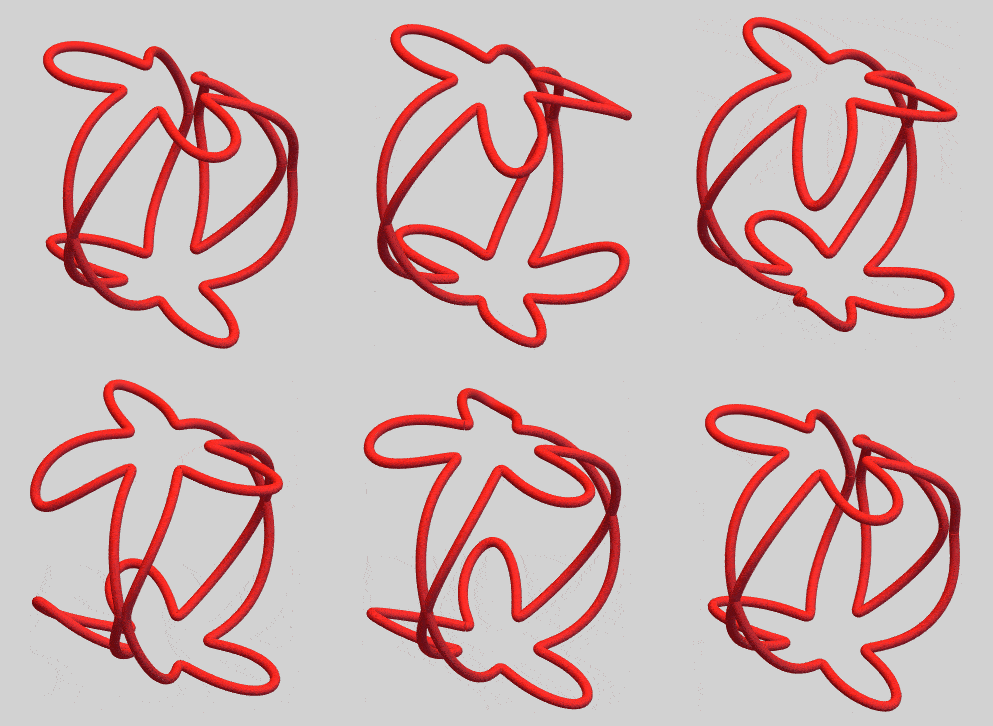
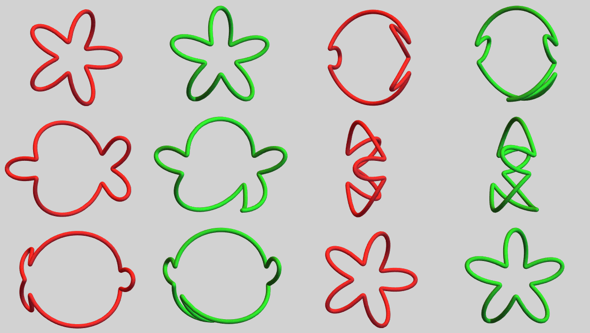
We can now put both animations together and demonstrate yet another example of shape-shifting in 3D:
This shows the "ambiguous" views that can be obtained while rotating the viewpoint around one of these 'shifted" shapes. Notice the circle and the 5-petaled rose views when the rotation is stopped briefly. These two views are at perpendicular view directions.
Selecting only half of this ringset will give an "ambiguous ring". This is a ring that can be seen as a rose or a circle, depending on the view direction. Two, almost perpendicular, view directions can be achieved by means of a mirror. An object in front of a mirror can be viewed either directly or reflected in the mirror. The two view directions form an almost right angle.
This is the code to generate and 3D-print these two ambiguous rings:
Module[{d, r, t1,
   t2, \[Theta]0}, {d, r, t1, t2, \[Theta]0} = {0,
    0.956394658621, -0.58857, 0.58857, -\[Pi]/2};
  roseRing51 =
   ParametricPlot3D[
    roseRing1CF[t, r, \[Theta]0, d, 5, 0., t1, t2], {t, -\[Pi], \[Pi]},
    PlotStyle -> {{Lighter[Red, .2], Tube[.065]}}, PlotPoints -> 200,
    PerformanceGoal -> "Quality", SphericalRegion -> True,
    PlotRange -> 1.08, Background -> Lighter[Gray, 0.65],
    ImageSize -> 300, Boxed -> False, Axes -> False]];
Printout3D[roseRing51, "Sculpteo", TargetUnits -> "Centimeters",
 RegionSize -> 5]

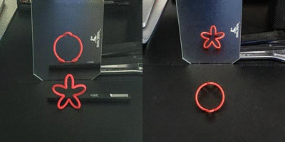
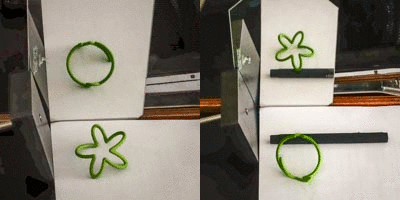
Now it is time to try these two ambiguous rings in front of a mirror and see the direct and the reflected views simultaneously. For each ring, we have two options :
direct view is a 5-petaled rose and reflected view is a circle (right photo)
direct view is a circle and reflected view is a 5-petaled rose (left photo)
The number of such "ambiguous rings" is almost unlimited and depends only on the cross sections of the intersecting cylinders. maybe the readers of this community can try their own unique combination!