First and foremost, all kudos go to Michael Trott for the original idea and coding composition. I found this fascinating example in Lou D'Andria's WTC talk presenting Manipulate for the first time. My work, i.e. presenting the code of the example in legible form with comments and updates, is fully based on his work and would not have been possible without it. It took me a total of 3 full days to untangle the code structure and do the minor revisions, now it is time to share. This example is a great instructive example demonstrating how a small set of Equations of Motion can be visualized in a graphics simulation (instead of a plot), how the implementation is actually carried out, elegantly in all its details. What makes this code so enjoyable to the beginner is that the underlying maths, programming concepts, and most coding details are very straight-forward and exemplary, with no convoluted algorithms involved. Any freshman student should be able to transfer the lessons learned here to similar problems (i.e. setting up the Equations of Motion and presenting the solution in an animated/interactive graphics) from his textbook. Thanks a mil and a big shout out to Michael for all his brilliant contributions to the community!
Separate note:
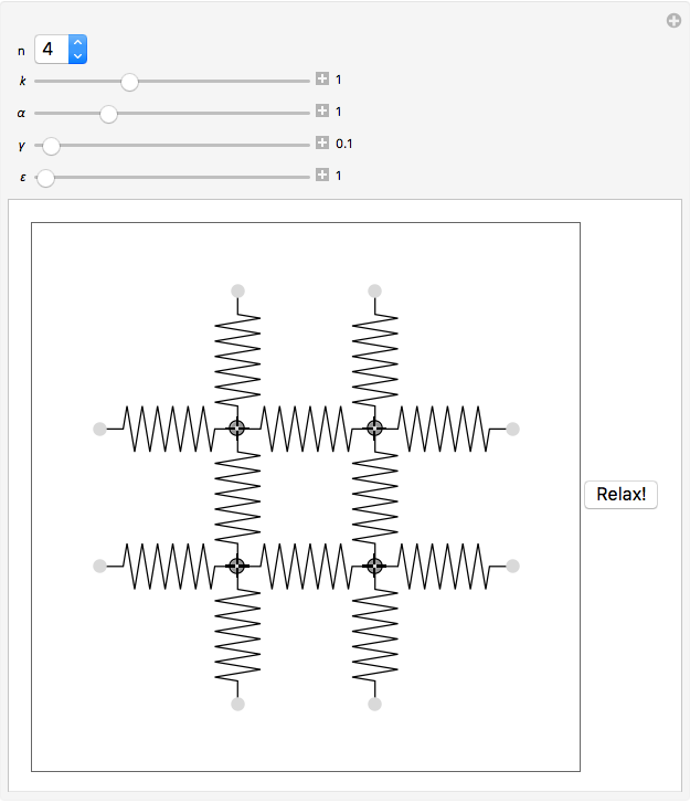
Btw this is really "just" an example, not a demo; you cannot find it on the Demonstrations webpage. Open the notebook file, no need to hit 'Evaluate Notebook' from your file menu; just scroll down to the output, shift the locators and click on the button. As you can see from the animated GIF, it takes some time, after pressing the "Relax!"-button, until the animation result window pops up. Complex computations take time! Because of eventual numerical instability and division-by-zero issues it is best to shift all mass points (locators), at least by a tiny bit, before clicking on the button. And the absolute shifts and parameter changes shouldn't be extreme either: be moderate with the shifts and changes! Again, the whole point is not to show that the program works but to learn how everything was put together, so masterfully, beautifully and straight-forward, with all the attention to detail.
Description
The code formatting loosely follows the convention introduced by Boris. We will use the value n=4 in our comments for exemplification purposes. This means that we are working with a 4x4 square grid whose bottom left corner has the Cartesian coordinates {0,0} and the top right corner {3,3}. There are no balls (or mass points) in the four corners of the square, the 2 balls at each edge (side) of the square are fixed, immobile. Coincidentally the number of mobile, inner grid balls is 4, too (in an n=3 grid there would be only 1 mobile ball, just saying).
We identify such a mobile ball through its grid index  with
with  , for a total of (n-2)(n-2) mobile balls. The current location, at any time t* , of an inner grid ball with respect to the global axes is
  , a pair of Cartesian coordinates. For identification purposes we must assign those indices to the coordinates as well
  meaning nothing but
  . The position (location) of each ball is measured with respect to the same single one "global" x-y-coordinate system. In other words, there are no other, individual fixed or individual moving (relative)
  -coordinate systems; the indices are used only to identify the object (or a grid point/position) and do not mean any different or individual coordinate system.
Now, it is obvious that every inner grid ball has four neighboring balls. If  is our center of attention (e.g. for setting up its F = m a equation) and its location is , then its four neighboring mass points are
  , and their respective locations are
  . We would not really need this function, but it makes the next function conciser and more intelligible. And it is always good programming practice to modularize parts of a larger code.
neighbors[{x[i_, j_][t_], y[i_, j_][t_]}] := (* or simply define as neighbors[i_,j_,t_]:= *)
 {
  {x[i + 1, j][t], y[i + 1, j][t]},
  {x[i - 1, j][t], y[i - 1, j][t]},
  {x[i, j + 1][t], y[i, j + 1][t]},
  {x[i, j - 1][t], y[i, j - 1][t]}
 }
We will also assume that every ball has the identical mass,  .
.
Vector Mechanics
If there is a spring connected between two points p1 and p2, then the spring force vector is certainly oriented in the vectorial direction between these two points. A tension spring exerts a pulling force, pulling at either point; a compression spring presses on either point. In the 1-D case, the algebraic signs in a textbook formulation like 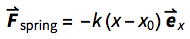 are dependent on the very orientation of the x-coordinate system at the time of formulation. In the 3-D case, using vector mechanics, we can formulate the spring force in a coordinate-free manner. The external force at point p1 be defined as a pulling force, pulling from p1 in direction to p2; in a linear relationship ( ? = 1), the magnitude of the force is proportional to the elongation:
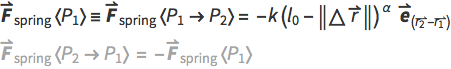
The direction of  is defined in a such a way that it always points from p1 (the focus of our attention) to p2 (which may be a neighboring point). In our setup, if the EuclideanDistance between p1 and p2 is 1, then the spring is in its relaxed state and the spring force is zero. If the distance exceeds 1 (i.e. p2 is far away from p1), the spring becomes a tension spring and the spring force is pulling at point p1 in that very direction. If the magnitude of undershoots 1 (i.e. p2 is very near to p1), then the spring becomes a compression spring and the spring force is pressing on our point p1. By introducing the parameter ? , we could deviate from the linear relationship between elongation and spring force. The formulation with Sign plus Abs is needed to circumvent problems with complex numbers resulting from a non-integer exponent ? .
springForce[{p1_, p2_}, \[ScriptK]_, ?_] :=
 (
  dp = p2 - p1;
  -Sign[1 - Norm[dp]]*\[ScriptK]*Abs[1 - Norm[dp]]^? * Normalize[dp]
 )
Assuming that there are no other external forces like gravitation or whatever, the modeling of the motion of a mass point is not complete until we introduce at least one term which covers damping. Damping could occur in the springs themselves, but to make our lives easier, we will assume that damping is caused only by friction with the surrounding air and that it is independent from the massless lossless springs. A textbook formulation, again dependent on the orientation of the coordinate system, would be 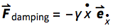 where the minus sign again helps to remind that the external force on the mass is opposite to the mass's motion. The general coordinate-free formulation with again introducing another parameter, ?, for minor non-linearity is:
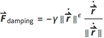
Putting the bits together, we are ready to write down the vector equation of motion F = m a . Since we are in 2-D space, for each mobile mass point there are two equations to solve: one ordinary differential equation for the x-component and one ODE for the y-component. For example, an n=4 grid with four mobile mass points will generate a system of eight coupled ODE's. (In comparison, an n=3 grid has only one mobile mass point and will generate two coupled ODE's.)

Implementing the maths
It is a common trick to reduce the order of an ODE by introducing new intermediary variables to solve for: the time derivative of the location vector is its velocity. Even though the resulting set of 16 coupled equations are not partial differential equations involving space derivatives, there are 16 "boundary conditions" to take into account. At any time t, the two mass points on each side (edge) are immobile, they do not displace, they do not have a velocity. Substituting these conditions reduces the complexity of the equations and is mandatory; without them the equations would not be solvable.
equationsOfMotion[
  n_, {\[ScriptK]_, ?_, ?_, ?_}] :=
 Table[
    {Thread[
      D[{x[i, j][t], y[i, j][t]}, t] == {vx[i, j][t], vy[i, j][t]}
      ]
     , Thread[
      D[{vx[i, j][t], vy[i, j][t]}, t] ==
       Total[
         springForce[{{x[i, j][t], y[i, j][t]}, #}, \[ScriptK], ?] &
          /@ neighbors[{x[i, j][t], y[i, j][t]}]
         ]
        - ?*Norm[{vx[i, j][t], vy[i, j][t]}]^? * Normalize[{vx[i, j][t], vy[i, j][t]}]
      ]
     }, {i, 1, n - 2} , {j, 1, n - 2} (*covers all inner points*)
    ] /. (* boundary conditions for left right bottom top edges at any time t *)
    {x[0, j_][_] :> 0 (* x-coord of left edge mass remains zero *)
    , y[0, j_][_] :> j (* y-coord of left edge mass is its initial grid location *)
    , x[n - 1, j_][_] :> n - 1 (* x-coord of right edge mass remains constant *)
    , y[n - 1, j_][_] :> j (* y-coord of right edge mass is its initial grid location *)
    , x[j_, 0][_] :> j (* x-coord of bottom edge mass is its initial grid location *)
    , y[j_, 0][_] :> 0 (* y-coord of bottom edge mass remains zero *)
    , x[j_, n - 1][_] :> j (* x-coord of top edge mass is its initial grid location *)
    , y[j_, n - 1][_] :> n - 1 (* y-coord of top edge mass is its initial grid location *)
    , vx[0, j_][_] :> 0 (* x-velocity of left edge mass remains zero *)
    , vy[0, j_][_] :> 0 (* y-velocity of left edge mass remains zero *)
    , vx[n - 1, j_][_] :> 0 (* x-velocity of right edge mass remains zero *)
    , vy[n - 1, j_][_] :> 0 (* y-velocity of right edge mass remains zero *)
    , vx[j_, 0][_] :> 0 (* x-velocity of bottom edge mass remains zero *)
    , vy[j_, 0][_] :> 0 (* y-velocity of bottom edge mass remains zero *)
    , vx[j_, n - 1][_] :> 0 (* x-velocity of top edge mass remains zero *)
    , vy[j_, n - 1][_] :> 0 (* y-velocity of top edge mass remains zero *)
    } // Flatten
Once you have the equations of motion, you only need to provide initial conditions, at time t=0, for all 16 variables to solve for. NDSolve produces a list of rules, so it is common procedure to use them as replacement rules. Even though we solve for 16 unknowns, in the end we are interested in 8 unknowns only, namely the locations (not the velocities) of the four mobile mass points.
solveEquationsOfMotion[xyInits_, vxyInts_, {\[ScriptK]_, ?_, ?_, ?_}, T_] :=
 Module[{n = Length[xyInits] + 2},
  Table[
    {x[i, j], y[i, j]} (*locations of the 4 mobile mass points*)
    , {i, 1, n - 2}
    , {j, 1, n - 2}
    ] /.
   NDSolve[
     {equationsOfMotion[n, {\[ScriptK], ?, ?, ?}]
       , MapThread[Equal
        , {
         Table[{x[i, j][0], y[i, j][0]}, {i, 1, n - 2}, {j, 1, n - 2}]
         , xyInits
        }, 3]
       , MapThread[Equal
        , {
         Table[{vx[i, j][0], vy[i, j][0]}, {i, 1, n - 2}, {j, 1, n - 2}]
         , vxyInts
        }, 3]
       } // Flatten
     , Table[{x[i, j], y[i, j], vx[i, j], vy[i, j]}, {i, 1, n - 2}, {j, 1, n - 2}] // Flatten
     , {t, 0, T}
    ][[1]]
  ]
Implementing the graphics
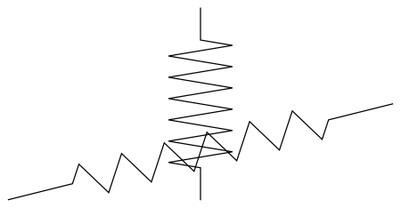
The following clever code generates a Line object which does indeed look like a spring in a graphical output. If you cannot come up with such an algorithm on your own (or cannot even understand how the below code works!), you could possibly find a similar code in a graphics generation handbook or an algorithm collection handbook or on the internet. In fact, even more sophisticated graphics could be generated.
springLine[{p1_, p2_}, w_] :=
 Module[
  {q1 = p1 + (1*(p2 - p1))/6
   , q2 = p2 + (1*(p1 - p2))/6
   , dq
   , l
   , m
  },
  dq = q2 - q1;
  l = Norm[dq];
  m = (Reverse[dq]*{-1, 1})/l;
  Line[{p1, q1, ##, q2, p2}] & @@ Table[
    q1 + (k/w + 1/(2*w)) dq + (-1)^k*m*Min[1/(8*l), 1/(w/2)]
    , {k, 0, w - 1}
    ]
  ]
w is the number of half-coils. We are going to use w = 12, so for our 6 full coils the non-trivial Line object will consist of 16 points. Generating a sequence of 16 points programmatically which will look like a spring, if connected in order, requires a brilliant mind and is beyond the scope of this walkthrough.
Graphics[{springLine[{{0, 0}, {2, 0.5}}, 12], springLine[{{1, 0}, {1, 1}}, 12]}]
The following function builds up the graphics for a snapshot in time. At time t of the solution, the locations of all mobile mass points are known. With this information we can create the graphics for the points and the springs. The mass points at the edges are immobile, hence their locations are always constant and do not depend on time.
springGraphics[ndsol_, t_] :=
 Module[{xyValues, mS, dQ, n = Length[ndsol] + 2},
  xyValues =
   Table[
    Which[
     i == 0, {0, j} (*location of grid points at the left edge is fixed*)
     , i == n - 1, {n - 1, j} (*location of grid points at the right edge is fixed*)
     , j == 0, {i, 0} (*location of grid points at the bottom edge is fixed*)
     , j == n - 1, {i, n - 1} (*location of grid points at the top edge is fixed*)
     , True, {ndsol[[i, j, 1]][t], ndsol[[i, j, 2]][t]} (*location of mobile mass points*)
     ], {i, 0, n - 1}, {j, 0, n - 1}
    ]

  ; mS[{i1_, j1_}, {i2_, j2_}] :=
   If[
    TrueQ[dQ[Sort[{{i1, j1}, {i2, j2}}]]]
    , {} (*gets rid of ugly multiple drawings of the same spring*)
    , dQ[Sort[{{i1, j1}, {i2, j2}}]] = True
    ; springLine[{xyValues[[i1, j1]], xyValues[[i2, j2]]}, 12]
   ]

  ; Graphics[
   {
    {PointSize[0.2/n]
     , Gray
     , Table[Point[{i, 0}], {i, 1, n - 2}] (*bottom 2 gray static points*)
     , Table[Point[{i, n - 1}], {i, 1, n - 2}] (*top 2 gray static points*)
     , Table[Point[{0, j}], {j, 1, n - 2}] (*left 2 gray static points*)
     , Table[Point[{n - 1, j}], {j, 1, n - 2}] (*right 2 gray static points*)
    },
    {PointSize[0.2/n]
     , Black (*inner 4 black mobile points*)
     , Table[Point[xyValues[[i + 1, j + 1]]], {i, 1, n - 2}, {j, 1, n - 2}]
    },
    Table[
     {Thickness[0.002]
      , Black
      , mS[{i + 1, j + 1}, {i + 1, j}] (*bottom edge springs*)
      , mS[{i + 1, j + 1}, {i + 1, j + 2}] (*all other vertical springs*)
      , mS[{i + 1, j + 1}, {i, j + 1}] (*left edge springs*)
      , mS[{i + 1, j + 1}, {i + 2, j + 1}] (*all other horizontal springs*)
     }, {i, 1, n - 2}, {j, 1, n - 2}
    ]
   }, PlotRange -> All
   , Frame -> True
   , FrameTicks -> None
   , PlotRangeClipping -> False
   ]
  ]
Combining maths and graphics in a Manipulate
The final function produces the interactive output where the user can move the locators with the mouse, thereby automatically setting the initial condition for the locations, i.e. the initial locations. The code assumes that the initial velocities are zero for all mobile mass points, both in the x-direction and y-direction. The programming is very straight-forward and clear, with no tricks or algorithms employed.
ManipulateSprings[] :=
 Manipulate[

  DynamicModule[
   {T = 100
    , xyValues
    , innerPositions
    , locators
    , pt
    , allSpringPointPairs
    , ndsol
   },
   xyValues =(*after deletion of 4 corners \[Rule] 12 grid coordinates left*)
    DeleteCases[#, {0, 0} | {0, n - 1} | {n - 1, 0} | {n - 1, n - 1}] &[
     Flatten[
      Table[{i, j}, {j, 0, n - 1}, {i, 0, n - 1}]
      , 1]
    ]

   ; innerPositions = Dynamic /@ (*list of the 4 mass ID's in 4x4 grid*)
     Flatten[
      Table[pt[{i, j}], {j, 1, n - 2}, {i, 1, n - 2}]
      , 1]

   ; locators = Locator /@ innerPositions (*4 locators in 4x4 grid*)

   ; Do[pt[{i, j}] = {i, j}, {j, 0, n - 1}, {i, 0, n - 1}](*initial coords*)

   ; allSpringPointPairs = (*12 spring locations in 4x4 grid*)
     Union[Sort /@
       Flatten[
        Table[
         {
          {{i, j}, {i, j - 1}}
          , {{i, j}, {i, j + 1}}
          , {{i, j}, {i - 1, j}}
          , {{i, j}, {i + 1, j}}
         }, {i, 1, n - 2}, {j, 1, n - 2}
        ]
        , 2]
     ]

   ; Row[{
      Graphics[
       {Dynamic[
         springLine[pt /@ #, 12] & /@ allSpringPointPairs
        ]
       , {PointSize[0.1/n], LightGray, Point[xyValues]} (*12 light gray markers*)
       , locators
      }
      , Axes -> False
      , Frame -> True
      , FrameTicks -> None
      , ImageSize -> 400
      , PlotRangeClipping -> False
      , PlotRange -> {{-0.5, -0.5 + n}, {-0.5, -0.5 + n}}
     ]
     , Button[
       "Relax!"
       , ndsol = solveEquationsOfMotion[
        Table[pt[{i, j}], {i, 1, n - 2}, {j, 1, n - 2}] (* interactive inital position of 4 masses *)
        , Table[{0, 0}, {n - 2}, {n - 2}] (* {{{0,0},{0,0}},{{0,0},{0,0}}} *)
        , {\[ScriptK], ?, ?, ?}
        , T]
      ; Animate[
        springGraphics[ndsol, t]
        , {t, 0, T, 0.25}
        , DisplayAllSteps -> True
        ] // CreatePalette
      , ImageSize -> Full
      , Method -> "Queued"
     ]
    }]
   ]
  (* and here are the 5 parameters available for manipulation: *)
  , {{n, 4}, {3, 4, 5, 6, 7, 8}}
  , {{\[ScriptK], 1}, 0.01, 3, Appearance -> "Labeled"}
  , {{?, 1}, 0.01, 4, Appearance -> "Labeled"}
  , {{?, 0.1}, 0.01, 4, Appearance -> "Labeled"}
  , {{?, 1}, 1, 4, Appearance -> "Labeled"}
  , SaveDefinitions -> True
  ]
As it turns out, the solver does not cope well with ? being less than 1, so the lower limit for this parameter be 1. Also, for very wild initial locations the solver may interrupt the calculation with a numerical error message. And the higher the computational load, the longer it takes until the animation is ready for playback.
Calling the program
ManipulateSprings[]
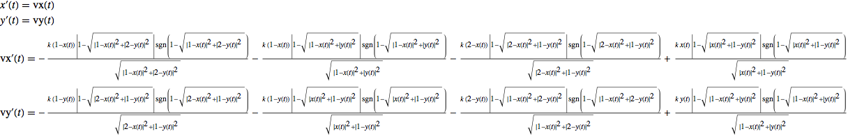
Here we can see that even for the simplest case, 1 single mobile mass point (n=3), the coupled equations of motions are already very complicated and impossible to solve without a computer.
test1 = equationsOfMotion[3, {\[ScriptK], ?, ?, ?}] /. {? -> 1, ? -> 0, ? -> 1};
test2 = test1 /. {x[1, 1] -> x, y[1, 1] -> y, vx[1, 1] -> vx, vy[1, 1] -> vy};
Column@test2 // TraditionalForm
This program is very instructive and likable because it shows how not trivial it is to go from a set of equations to the actual implementation, doing both the maths and the graphics, not just a simple plot. Many details need to be taken care of during the implementation, most of which a beginner would not have thought of. Maybe the most challenging part was the juggling with the iterators i and j, getting them right in the various Table statements and also not to get confused by the multiple curly braces in intermediary output expressions. It is amazing how the Wolfram Language can express massive sets of long confusing equations in a very succinct clear form, almost as elegantly as a vector mechanics equation. Now i want to see this problem solved in any other language! :D
 Attachments:


