After some detailed experiments with C++ code, the bimodal behavior and switching between the two local maxima (in terms of reporting the maximum) has the flavor of Chebyshev equioscilation that is obtained via minimax algorithms. In fact I am trying to do some error balancing, and the u-parameter is what I vary to do the balancing. When you remove the Abs[] from g[...] and call Plot3D as I did, you get a local minimum (on boundary) and a local maximum (in the interior) that have same magnitude but opposite sign (within numerical rounding errors in the code). The difference between the C++ results and the Mathematica results is that the C++ code makes it clear that when one local maxima becomes smaller than the other as u varies past the switching point, the magnitudes are nearly the same.

Thanks for your input. Perhaps someone will eventually help me with those Mathematica errors when I don't use NumericQ.

With the NMinimize function included, the reported value is u=0.852.

That said, I tracked down the problem. To compare with my C++ results, where I use a dense sampling of (x,t) for each u in a set of 1024 and select the maximum, I used

ListLinePlot[Table[{u, h[8, u]}, {u, 0.8519, 0.8521, 0.0002/1024}]]

The output image is

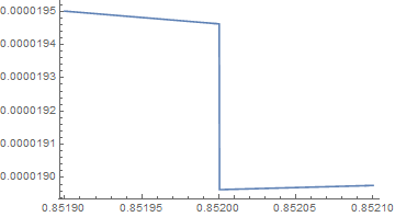
which makes it appear that there is a discontinuity at u = 0.852. The call

NMaximize[{g[8, 0.8519, x, t], 0 <= x <= 1 && 0 <= t <= 1}, {x, t}, Method -> "DifferentialEvolution"]

produces {0.0000195003, {x -> 0., t -> 0.476764}} and the call

NMaximize[{g[8, 0.8521, x, t], 0 <= x <= 1 && 0 <= t <= 1}, {x, t}, Method -> "DifferentialEvolution"]

produces {0.0000189766, {x -> 0.129624, t -> 0.521673}}. The result for u = 0.8521 is what I believe to be incorrect (and in fact incorrect for any u > 0.852 in the line-list plot). I called

Plot3D[g[8, 0.8521, x, t], {x, 0, 1}, {t, 0, 1}, PlotRange -> All, PlotPoints -> 50]

which generated the output

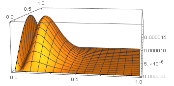
so the graph is bimodal. For u=0.8251, NMaximize reports the local maximum at (x,t)=(0.129624,0.521673). The local maximum on the boundary x=0 occurs at t=0.476541 and the value is 0.000019424, which is larger than the local maximum in the interior. I obtained the boundary computation from

NMaximize[{g[8, 0.8521, 0, t], 0 <= t <= 1}, t, Method -> "DifferentialEvolution"]

I mentioned in my post that I omitted the final line of the minimax operation. After the definition of h[n_,u_] my actual code has

hmin = NMinimize[{h[8, u], 0 <= u <= 1}, u]

Without the NumericQ, this generates several lines of errors "... NMaximize: The function value 0 is not a number at (t,x) = {0.918621,0.831757}" followed by "...General: Further output of NMaximize::nnum will be suppressed during this calculation." and the NMinimize fails (but the ListLinePlot succeeds). My goal is to obtain the minimum and where it occurs. Is there some way to avoid these errors? With NumericQ and the NMinimize line included, the program ran for over 2 hours (on a high-end desktop computer, but Mathematica appeared to be using 20% CPU [about 2 logical processors]) . Also, your code shows the same numerical anomalies when NMaximize uses its default method.

Thank you.