NOTE: originally posted in response to: http://community.wolfram.com/groups/-/m/t/1398247
Related Notebooks
There are a couple of Mathematica notebooks related to chromatography that you may find useful. The first is from Professor Brian Higgins called ChromatographyAnalysis.nb from his Ekaya Solutions website. The website has a plethora of Mathematica notebooks related to chemical engineering. If you have Wolfram SystemModeler, there is a Chromatography Example Model from the Wolfram website.
Basic Problem
To get the behavior that you desire, there is an implied step function that is missing from the equations that you posted. For "irreversible" adsorption, the time derivative of adsorbate loading must equal 0 at saturation. We also know that the solute concentration should be highest when the media is saturated. You will need to add a step function to drive the time derivative of W to be 0 at saturation. The result will be a phase boundary that moves and your equations are only valid for solid that is unsaturated. Therefore, the domain shape will be a function of time. I believe that this will mean that there are no analytical solutions available from DSolve and that you will need to use NDSolve to solve the system of PDEs. Traditionally, one would make a quasi-steady-state assumption and use a saturated moving boundary to obtain an approximate solution. I think an NDSolve solution will be instructive to show how the bed evolves over time and potentially give insights on simplified models.
Dimensional Analysis
If you will indulge me for a moment, I would like to make the system of equations dimensionless so that we reduce the dependence to a minimum number of meaningful dimensionless groups with variables that have a nice scale.
There is a fluid phase and a solid phase in your system, so it makes sense that there should be a state variable for each phase. Our initial system of PDEs is given by:
$$\begin{gathered} \varepsilon \frac{{\partial {c_d}}}{{\partial {t_d}}} + \left( {1 - \varepsilon } \right){\rho _p}\frac{{\partial {W_d}}}{{\partial {t_d}}} = - u\frac{{\partial {c_d}}}{{\partial {x_d}}} \qquad (1) \\ \left( {1 - \varepsilon } \right){\rho _p}\frac{{\partial {W_d}}}{{\partial {t_d}}} = {K_c}a\left( {{c_d} - c_d^*} \right) \qquad (2) \\ \end{gathered}$$
I added a subscript d to indicate that there are dimensions associated with those variables.
Next, to make variables dimensionless, simply divide the dimensioned variables by characteristic dimensions. For characteristic time, we will use the convective timescale or:
$$\begin{gathered} {\tau _c} = \frac{{\varepsilon L}}{u} \\ t = \frac{{{t_d}}}{{{\tau _c}}};{t_d} = {\tau _c}t \\ x = \frac{{{x_d}}}{L};{x_d} = Lx \\ c = \frac{{{c_d}}}{{{c_0}}};{c_d} = {c_0}c \\ w = \frac{{{W_d}}}{{{W_{sat}}}};{W_d} = {W_{sat}}w \\ \end{gathered}$$
Now, let's return to equation (1) and make the appropriate substitutions. $$\frac{\varepsilon }{{{\tau _c}}}{c_0}\frac{{\partial c}}{{\partial t}} + \left( {1 - \varepsilon } \right){\rho _p}\frac{{{W_{sat}}}}{{{\tau _c}}}\frac{{\partial W}}{{\partial t}} = - \frac{{u{c_0}}}{L}\frac{{\partial c}}{{\partial x}}\left\| {\frac{{\varepsilon L}}{u}} \right.\frac{1}{{\varepsilon {c_0}}}$$
Perform some algebra $$\begin{gathered} \frac{\varepsilon }{{{\tau _c}}}\frac{L}{{u{c_0}}}{c_0}\frac{{\partial c}}{{\partial t}} + \left( {1 - \varepsilon } \right){\rho _p}\frac{{{W_{sat}}}}{{{\tau _c}}}\frac{{\varepsilon L}}{u}\frac{1}{{\varepsilon {c_0}}}\frac{{\partial w}}{{\partial t}} = - \frac{{\partial c}}{{\partial x}} \\ \frac{{\partial c}}{{\partial t}} + \frac{{\left( {1 - \varepsilon } \right)}}{\varepsilon }\frac{{{\rho _p}}}{{{c_0}}}{W_{sat}}\frac{{\partial w}}{{\partial t}} = - \frac{{\partial c}}{{\partial x}} \\ m = \frac{{\left( {1 - \varepsilon } \right)}}{\varepsilon }\frac{{{\rho _p}}}{{{c_0}}}{W_{sat}} \\ \boxed{\frac{{\partial c}}{{\partial t}} + m\frac{{\partial w}}{{\partial t}} + \frac{{\partial c}}{{\partial x}} = 0} \\ \end{gathered}$$
The boxed formula represents the dimensionless version of (1). The dimensionless group, m, can be thought of as a loading factor (i.e., how much the adsorbant bed can adsorb versus the incoming concentration $c_0$. Now, we continue with equation (2). $$\begin{gathered} \left( {1 - \varepsilon } \right){\rho _p}\frac{{{W_{sat}}}}{{{\tau _c}}}\frac{{\partial w}}{{\partial t}} = {K_c}a{c_0}\left( {c - {c^*}} \right)\left\| {\frac{{{\tau _c}}}{{\varepsilon {c_0}}}} \right. \\ \frac{{\left( {1 - \varepsilon } \right)}}{\varepsilon }\frac{{{\rho _p}}}{{{c_0}}}{W_{sat}}\frac{{\partial w}}{{\partial t}} = \frac{{{K_c}a}}{\varepsilon }{\tau _c}\left( {c - {c^*}} \right) \\ m\frac{{\partial w}}{{\partial t}} = \frac{{{\tau _c}}}{{{\tau _a}}}\left( {c - {c^*}} \right);{\tau _a} = \frac{\varepsilon }{{{K_c}a}};n = \frac{{{\tau _c}}}{{{\tau _a}}} \\ \boxed{m\frac{{\partial w}}{{\partial t}} = n\left( {c - {c^*}} \right)} \\ \end{gathered} $$
The boxed formula represents the dimensionless version of (2). The new dimensionless group, n, can be thought of as the ratio of the convective time scale to the adsorption time scale.
Your system of PDEs for irreversible adsorption in dimensionless terms would be:
$$\begin{gathered} \frac{{\partial c}}{{\partial t}} + m\frac{{\partial w}}{{\partial t}} + \frac{{\partial c}}{{\partial x}} = 0 \qquad (3) \\ m\frac{{\partial w}}{{\partial t}} = nc \qquad (4) \\ \end{gathered} $$
To correct equation (4) for the "equilibrium" condition of ${\left. {\frac{{\partial w}}{{\partial t}}} \right|_{w = 1}} = 0$ , we will need add a unit step function, $\theta$, to drive the time derivative to 0 at saturation and bringing over the left hand side of the equation or:
$$m\frac{{\partial w}}{{\partial t}} - nc\theta (1 - w)=0\qquad(4*)$$
Bed Saturation Start-up Transient
If we start with a clean bed, it will take some time before the bed saturates at $x=0$. We can use equation (4) evaluated at $x=0$ to determine the time to initially saturate the front of the bed.
$$m{\left. {\frac{{\partial w}}{{\partial t}}} \right|_{x = 0}} = nc_0=n\qquad Conditions = \left\{ {\begin{array}{*{20}{c}} {IC}&{w(t = 0,x = 0) = 0} \\ {FC}&{w(t = {t_{sat}},x = 0) = 1} \end{array}} \right\}$$
$$w(t,x=0)=\frac{n}{m}t$$ $$\therefore t_{sat}=\frac{m}{n}$$
We can check our NDSolve solutions to verify that they approximate this relation.
Mathematica Implementation
We should be able to use NDSolve to solve this system of PDEs. I had some performance issues with UnitStep[] so I opted to use the Tanh[] function to create a sharp, but differentially continuous approximation to the UnitStep[] function. Perhaps, there is a more elegant Mathematica implementation, but the Tanh[] functions seems to be working for $m$ and $n$ < 20.
Finally, we need two initial conditions (the bed and liquid is initially free of adsorbate species) and one boundary condition (a "UnitStep" of species at the inlet).
The initial conditions:
$$\begin{gathered} c[0,x] = 0 \\ w[0,x] = 0 \\ \end{gathered} $$
The boundary condition:
$$c[t,0] = \tanh (200t)$$
This yields the following set of equations.
eqn1 = D[cp[t, x], t] + m D[wp[t, x], t] + D[cp[t, x], x] == 0;
eqn2 = m D[wp[t, x], t] -
    n  cp[t, x] (1 - (1 + Tanh[200 (wp[t, x] - 1)])/2) == 0;
ics = {wp[0, x] == 0, cp[0, x] == 0};
bcs = {cp[t, 0] == Tanh[200 t]};
eqns = {eqn1, eqn2} ~ Join ~ ics ~ Join ~ bcs;
opts = Method -> {"MethodOfLines",
    "SpatialDiscretization" -> {"TensorProductGrid",
      "MinPoints" -> 5000}};
The dimensional analysis says that this system of equations depends on only two dimensionless parameters suggesting that ParametricNDSolveValue[] might be the flavor of NDSolve[] to use. To resolve the sharp features, we will specify a large number of spatial points as shown in opts and a small timestep as shown below to return a parameteric function, pfun.
pfun = ParametricNDSolveValue[
   eqns, {cp, wp}, {t, 0, 10}, {x, 0, 1.1}, {m, n}, opts,
   MaxStepFraction -> 1/1000];
With a parametric function, it is easy to return an interpolation function, ifun, based on the parameters $m$ and $n$. We will set the loading factor, $m$, to 5 and the convective timescale to adsorption timescale, $n$, to 10 (we want the adsorption to be fast relative to convection). The following takes a couple of minutes to run on my machine.
ifun = pfun[5, 10];
c = ifun[[1]];
w = ifun[[2]];
We can plot the particular solution of the fluid solute concentration, $c(t,x)$, with Plot3D[].
Plot3D[Evaluate[{c[t, x]}], {x, 0, 1}, {t, 0, 10},
 PlotRange -> All, PlotPoints -> {200, 200},
 ColorFunction -> (ColorData["DarkBands"][#3] &),
 MeshFunctions -> {#2 &}, Mesh -> 20, AxesLabel -> Automatic,
 MeshStyle -> {Black, Thick}, ImageSize -> Large]
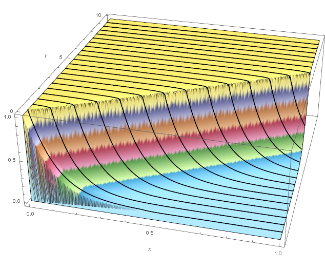
We see some discontinuities at small $t$ as the bed starts loading to saturation. We can zoom into the small $t$ and $x$ for a clearer picture.
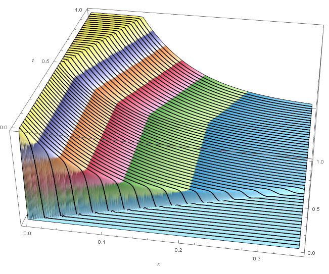
Plot3D[Evaluate[{c[t,x]}], {x, 0, 0.35}, {t, 0, 1},
 PlotRange -> All, PlotPoints -> {200, 200},
 ColorFunction -> (ColorData["DarkBands"][#3] &),
 MeshFunctions -> {#2 &}, Mesh -> 50, AxesLabel -> Automatic,
 MeshStyle -> {Black, Thick}]
We predicted that the bed at $x=0$ should staturate at $t=\frac{m}{n}=\frac{5}{10}=0.5$ and the plot does indicate that the bed does indeed begin to saturate at the predicted time. We also see that the bed saturation front grows linearly in time. Also, post saturation, the concentration falls off approximately exponentially with $x$ at constant time from the saturation boundary. Prior to initial saturation, the MeshFunctions curves do not appear that they can be described by simple functions. Even if a DSolve solution existed, it probably would not have a simple form.
A countour plot of $w$ and $c$ after initial saturation may give us some insights to a simplified model. The first contour plot is of the solid loading.
ContourPlot[
 Evaluate[{w[t + m/n, x]}], {x, 0, 5/(m + 1.3)}, {t, 0, 5},
 ColorFunction -> "DarkBands", Mesh -> 40, MeshFunctions -> {#3 &},
 FrameLabel -> {"x", "t"}, ImageSize -> Large]
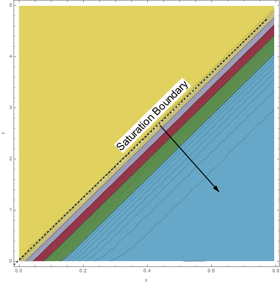
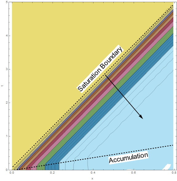
A remarkably linear Saturation Boundary forms after $t=\frac{m}{n}$. The contour lines look essentially parallel implying that we might model $w$ as function of a single variable perpendicular to the phase boundary. The concentration countour plot looks similar but there is an accumulation error that grows linearly in time.
ContourPlot[
 Evaluate[{c[t + m/n, x]}], {x, 0, 5/(m + 1.3)}, {t, 0, 5},
 ColorFunction -> "DarkBands", Mesh -> 40, MeshFunctions -> {#3 &},
 PlotRange -> {0, 1}, FrameLabel -> {"x", "t"}, ImageSize -> Large]
If we restrict the domain to only consider the unsaturated bed, then we can eliminate $w$ by combining equations (3) and (4) because the UnitStep function containing $w$ can be ignored.
$$\begin{gathered} \frac{{\partial c}}{{\partial t}} + m\frac{{\partial w}}{{\partial t}} + \frac{{\partial c}}{{\partial x}} = 0 \qquad (3) \\ m\frac{{\partial w}}{{\partial t}} = nc \qquad (4) \\ \\ \frac{{\partial c}}{{\partial t}} + \frac{{\partial c}}{{\partial x}}+ nc = 0 \qquad (5) \end{gathered} $$
You can use Mathematica to evaluate the partial derivatives somewhere in the unsaturated region to assess their magnitudes.
D[c[t, x], t] /. {t -> 2.5, x -> 0.4} (*0.8176759782035153`*)
D[c[t, x], x] /. {t -> 2.5, x -> 0.4} (*-4.995343977849113`*)
Mathematica suggests that the spatial derivative is much larger in absolute magnitude than the time derivative. We could make the pseudo steady-state assumption and (5) becomes a simple first order ODE as shown in (6).
$$\frac{{\partial c}}{{\partial x}} + nc = 0 \qquad (6) $$
More rigorously, but still approximately, we could try a transformed coordinate system as depicted in the diagram below so that the moving boundary line given by $t=m x + \frac{m}{n}$ coincides with the ${t}'$ axis. In this reference frame, (5) should depend only on one independent variable ${x}'$ and the moving boundary goes away.
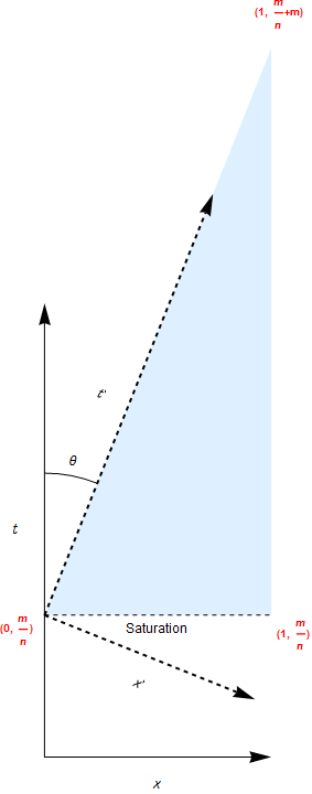
To transform $(x,t)\rightarrow ({x}',{t}')$ we can use Mathematica's Transform functions to first rotate the original coordinate system by $-\theta=ArcTan[m,1]$ then translate up to $\frac{m}{n}$. Transformations can always be confusing so it is good to have a check to see if the transform is valid. In the transformed coodinates, the moving boundary line should simply be ${x}'=0$ .
theta = ArcTan[m, 1];
rt = RotationTransform[-theta];
tt = TranslationTransform[{0, m/n}];
trf = tt@*rt;
tr = trf@{xp, tp} // Simplify;
rules = Thread[{x, t} -> tr];(*{x -> (tp + m*xp)/Sqrt[1 + m^2], t -> m*(n^(-1) + tp/Sqrt[1 + m^2]) - xp/Sqrt[1 + m^2]}*)
We can apply the transformation rules to the moving boundary line to show that indeed ${x}'=0$.
(t == m x + m/n) /. rules // Simplify (*Sqrt[1 + m^2]*xp == 0*)
But we want the inverse transform to get ${x}'$ in terms of $x$ and $t$, which we can obtain with the InverseFunction[].
invtrf = InverseFunction[trf];
invtr = invtrf@{x, t} // Simplify;
invrules = Thread[{xp, tp} -> invtr] // InputForm
(*{xp -> (m - n*t + m*n*x)/(Sqrt[1 + m^2]*n), tp -> (-m^2 + m*n*t + n*x)/(Sqrt[1 + m^2]*n)}*)
Revisting (5), we will combine the $x$ and $t$ variables into one independent variable ${x}'$ using the chain rule as shown below:
\begin{gathered} \frac{{\partial c}}{{\partial t}} + \frac{{\partial c}}{{\partial x}} + nc = 0; \ \frac{{\partial x'}}{{\partial t}}\frac{{\partial c}}{{\partial x'}} + \frac{{\partial x'}}{{\partial x}}\frac{{\partial c}}{{\partial x'}} + nc = 0; \ \left( {\frac{1}{n}} \right)\left( {\frac{{\partial x'}}{{\partial t}} + \frac{{\partial x'}}{{\partial x}}} \right)\frac{{\partial c}}{{\partial x'}} + c = 0 \ \end{gathered}
Mathematica can evaluate and simplify the change of variables derivatives as shown below.
1/n (D[#, t] + D[#, x]) & [xp /. invrules] // Simplify (*(-1 + m)/(Sqrt[1 + m^2]*n)*)
Leaving us with equation (7) and the corresponding solution (we could use DSolve, but the solution to this ODE is straightforward).
$$\begin{gathered} \frac{{m - 1}}{{n\sqrt {1 + {m^2}} }}\frac{{dc}}{{dx'}} + c = 0 \qquad (7) \\ c({x}')=e^{-\frac{n\sqrt{1+m^{2}}}{m-1}{x}'} \\ \end{gathered}$$
We can substitute and simplify $x$ and $t$ for ${x}'$ using the $invrules$ previously defined.
E^(-((Sqrt[1 + m^2]*n*xp)/(-1 + m))) /. invrules // InputForm (* E^(-((m - n*t + m*n*x)/(-1 + m))) *)
We recognize that $c$ is only defined to the right of the moving boundary to obtain the following piecewise function.
$$c(t,x)=\begin{Bmatrix} e^{\frac{n \left(\left(t-\frac{m}{n}\right)- m x\right)}{m-1}} & m x>t-\frac{m}{n}\\ 1 & \text{True} \end{Bmatrix}$$
If you wanted to wrap the whole process in one Mathematica call, you could do something like the following.
cc[xp /. invrules] /. First@DSolve[{
     (1/n (D[#, t] + D[#, x]) & [xp /. invrules]) D[cc[xp], xp] +
       cc[xp] == 0,
     cc[0] == 1},
    cc,
    xp
    ] // InputForm (* E^(-((m-n*t+m*n*x)/(-1+m))) *)
We will now create a function called breakthrough for the simplified model and a plotting function to compare the simple model to the result obtained by ParametricNDSolveValue[].
(* Simplified model *)
breakthrough[m_, n_, t_, x_] :=
 Piecewise[{{Exp[n ((t - m/n) - m x)/(m - 1)], m x > (t - m/n)}, {1,
    True}}]
(* Plot function to compare simplified model to NDSolve for given m,n, and t *)
pltfn := Plot[{Callout[breakthrough[#1, #2, #3, x], "Model", (
      Log[2] (-1 + #1) - #1 + #2 #3)/(#1 #2),
      CalloutMarker -> "CirclePoint"],
     Callout[c[#3, x], "NDSolve", (
      Log[2] (-1 + #1) - #1 + #2 #3)/(#1 #2),
      CalloutMarker -> "CirclePoint"]}, {x, 0, 1},
    PlotRange -> {0, 1.05}, Filling -> {1 -> {2}}, Exclusions -> None,
     PlotStyle -> Thick, Frame -> True,
    FrameLabel -> {Style["x", 18], Style["c(t,x)", 18],
      Style[StringForm["m=``, n=``, and t=``", #1, #2,
        NumberForm[#3, {2, 1}, NumberPadding -> {" ", "0"}]], 18]},
    ImageSize -> Large] & ;
(* Create a series of images at different times for animation *)
plts := Table[pltfn[#1, #2, t], {t, #1/#2, 10, 0.1}] &;
Here is an animation of the current solution for $m=5$ and $n=10$.
Export["510.gif", plts[5,10], "AnimationRepetitions" -> \[Infinity]]
The accumulation term causes NDSolve to lag our simple model. At larger $m$ and $n$ values, this lag is reduced. It is easy to insert $m=20$ and $n=10$ into our parametric function and animate the result to verify the accumulation lag is reduced. Now, the simple model approximates well the NDSolve solution.
ifun = pfun[20, 10];
c = ifun[[1]];
Export["2010.gif", plts[20, 10],
 "AnimationRepetitions" -> \[Infinity]]
Summary
- One needs to add a "UnitStep" function to stop adsorption when the bed becomes saturated.
- This will create a moving boundary meaning that the shape of the domain changes with time.
- Probably means DSolve will not find a solution.
- Dimensional analysis simplifies the equations and reduces the number of parameters that the equations depend on.
- ParametricNDSolveValue[] can be used to solve the system of PDEs.
- Using Plot3D and ContourPlot, we gain insights on a simplified model for the moving boundary.
- We can use Mathematica's Transform functions to create a new coordinate system that is perpendicular to the moving saturation boundary creating a simple solvable ODE.
- We created a simple model that tracks the results of NDSolve and the model should only get better at larger $m$ and $n$ values.


