Message Boards Message Boards

4
|
15746 Views
|
6 Replies
|
30 Total Likes
View groups...
Share
Share this post:

Modeling Financial Returns with Stable 2:3 Order Statistic Distribution

Posted 11 years ago
I have put up a series of webpages built from Mathematica notebooks, describing a new idea about how to model price returns:

Financial Data Analysis
 

The Mathematica notebook for each page may be downloaded and explored in detail.  There is a notebook which can be used to fit the stable 2:3 OrderDistribution. 

The central idea, which needs more more research, is that the process of price formation is driven by the two-tailed power law distribution in the limit order books of the continuous double auction .  Research has shown that this distribution is heavy tailed.  The thought is that a price formation distribution might arise from summation of the random variables found in the order book log return distribution across slices of time.  The limiting distribution would be a stable distribution having alpha determined by the lowest alpha in the order book distribution.  But this resulting price formation would be a distribution of prices which potentially could occur.  The distribution of prices which ultimately flow from the CDA would be a subset of these price log returns. 

A way to get this subset while resolving the tension between buyers and sellers would be to assume symmetry in the expectations of buyers and sellers and that they might each submit order prices with an expectation that half of the orders will never be executed.  The prices in the price formation  distribution which are actually executed would then come from the middle third of the distribution where the buyer and seller prices (modelled as log returns)  overlap.  The way to get the random variables for this distribution might be to sort the random variables from the price formation distribution, taking them three at a time and selecting the median return.  If the price formation distribution resulting from sums of returns across slices of time from the limit orders is a stable distribution then then the distribution of price returns might be well modeled by a stable 2:3 order statistic distribution. 

I try to articulate this better on this page:

A Market Thought Experiment

The fits to financial log returns to this distribution are remarkably good even at the one minute level, and it seems the hypothesis here could be tested by analyzing a source of high frequency level II quotes.  I don't have access to that but if anyone is interested in researching the idea I would be happy to collaborate.
POSTED BY: Robert Rimmer
6 Replies
Posted 11 years ago
Thanks for the interesting comments. It would be nice to have some actual order book data to play with. Perhaps someone with the Financial Platform hooked to a Bloomberg terminal could do that. Regarding order size, the idea is to keep the model simple. Varying order sizes can be simply added by putting in sequential runs of the same order, and the run lengths need not have a Poisson distribution. Looking at trading monitors, currently most all the transactions seem to be in small blocks, probably because orders are being split to prevent price impact.

Empirical distributions are fine as long as you want to stick to the time frame of the data, but if you want to scale them over different time frames, they will almost never get the tail behavior right, because of small number of data points in the tail. So to get the tail behavior it is almost necessary to have a model, but unless a model is very close to reality or you can prove it to be correct, it probably won't be reliable.

For instance the fit of the stable 2:3 order statistic distribution to the IBM example is quite good far out on the tails.
ibmprice=FinancialData["IBM",{2003,11,10},"Value"];
ibmlr=Differences[Log[ibmprice]];

parm = Quiet@S23MLFit[ibmlr, {3, 0, 0.01, 0}]
{2.49166, -0.0104217, 0.0107371, 0.000238817}

empD=EmpiricalDistribution[ibmlr];
mx=Max[Abs[ibmlr]];
LogLogPlot[{CDF[empD,-x],1-CDF[empD,x],CDF[S23OrderDistribution[Sequence@@parm],-x],
1-CDF[S23OrderDistribution[Sequence@@parm],x]},{x,0.001,mx},
PlotRange->All,PerformanceGoal->"Speed",Frame->True,GridLines -> Automatic,
PlotStyle->{Darker[Blue],Darker[Red],Darker[Blue],Darker[Red]},
PlotLabel-> "Tail Fit IBM with Empirical Distribution"]


So it is probably useful, but it would be nice to have a theoretical basis before using it.
POSTED BY: Robert Rimmer
This is an example of using SmoothKernelDistribution to model stock price returns as discussed in the thread.

To download Mathematica notebook: CLICK HERE

Get some stock data for IBM over the last 10 years

ibm = FinancialData["IBM", "FractionalChange", {2003, 11, 10}, "Value"];
ibmprice = FinancialData["IBM", {2003, 11, 10}, "Value"];

ListLinePlot[ibmprice, Filling -> Bottom, PlotRange -> All]


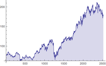
ibmfromchanges = FoldList[#1*(1 + #2) &, ibmprice[[1]], ibm];
ListLinePlot[{ibmprice, ibmfromchanges}, Filling -> Bottom, PlotRange -> All]


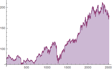
That was just to show we can use the FractionalChange property and it gives us single day returns, including dividends.
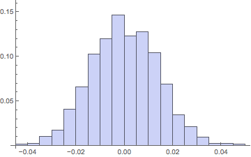

Return histogram

Histogram[ibm, {.005}, "Probability"]


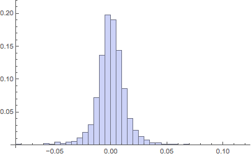
Note the high peak and long tails, with much less weight in the midrange flanks than in a normal distribution.


Basic descriptive statistics

In[]  = {Mean[#], StandardDeviation[#], Skewness[#], Kurtosis[#]} &@ibm
Out[] = {0.000428635, 0.0135803, 0.0600238, 9.54613}

Note the high figure for the Kurtosis - a Gaussian distribution would show a 3.00 on that measure.
In[] = aveannualreturn = (1 + Mean[ibm])^251 - 1
Out[] = 0.113562

we can annualize the return using 251 market days in the average year.
In[] = aveannualvolatility = (StandardDeviation[Log[1 + ibm]])*Sqrt[251.]
Out[] = 0.215138

For volatility, we annualize using the serial independence assumption, which implies the variation grows as the square root of the time. We have to use log returns to be symmetric in our treatment of proportional rises and falls.


SmoothKernel vs LogNormal

 ibmSKDist = SmoothKernelDistribution[Log[1 + ibm]];
 
 In[] = E^Mean[ibmSKDist] - 1
 Out[] = 0.000336473
 
 In[] = E^Mean[ibmSKDist] - 1
 Out[] = 0.000336473
 
 ibmLNDist = LogNormalDistribution[Sequence @@ params];

In[] = Length[ibm]
Out[] = 2517


SK sample

SKsample = E^RandomVariate[ibmSKDist, 2517] - 1;

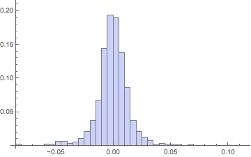
Histogram[SKsample, {.005}, "Probability"]


In[] = {Mean[#], StandardDeviation[#], Skewness[#], Kurtosis[#]} &@SKsample
Out[] = {-0.000258464, 0.0141158, -0.239577, 9.56601}

In[] = {Mean[#], StandardDeviation[#], Skewness[#], Kurtosis[#]} &@ibm
Out[] = {0.000428635, 0.0135803, 0.0600238, 9.54613}

Notice the excellent agreement of the smooth kernel distribution with the actual returns on Kurtosis and overall shape of the return histogram. But with only a single sample of the same length taken, the mean can easily "miss" by a significant amount.
In[] = Mean[E^RandomVariate[ibmSKDist, 2517000] - 1]
Out[] = 0.000439987

It is easy to get excellent agreement on the Mean as well by just using 1000 sample runs of the same length, rather than just one.


LN sample

LNsample = RandomVariate[ibmLNDist, 2517] - 1;

Histogram[LNsample, {.005}, "Probability"]


In[] = {Mean[#], StandardDeviation[#], Skewness[#], Kurtosis[#]} &@LNsample
Out[] = {0.000107968, 0.0137806, 0.057543, 2.92288}

In[] = {Mean[#], StandardDeviation[#], Skewness[#], Kurtosis[#]} &@ibm
Out[] = {0.000428635, 0.0135803, 0.0600238, 9.54613}

Notice, the lognormal distribution is able to get the first 3 moments of the distribution approximately correct, but the 4th - Kurtosis - is hopelessly low and the return histogram looks nothing like the real one as a result. It has way too much weight in the midrange flanks and not nearly enough in the small-change peak of the distribution.
POSTED BY: Jason Cawley
There are two additional points that I would make: When fitting to observed data there are two possible approaches: theoretical and empirical. From the point of view of a mathematician you may want to construct a model of the market that would allow for delta-gamma hedging and in that case it is better to have a well specified distribution with known properties. In that case Stable distributions are generalizations of the usual Normal/Lognormal models that lend themselves to further theoretical details. Research journals especially like this approach and we are all bound to publish or perish. But if your interests are solely empirical then the use of either EmpiricalDistribution[] or SmoothKernelDistribution[] will give an adequate description of the data for the purposes of trading and categorization.

In 1994 (I think) I presented a couple conference papers using the stable distribution as a method of analysis of market data just before the crash of 1987. It showed that just before a crash the market prices bifurcated and became bi- and even multi-modal so that the usual processes of market clearing broke down rapidly. These results are also predictable using Chaos theory. Even though the results were factual, I had a hard time getting it accepted because it showed that the market was not even weakly rational as hypothesized by the recent Nobel prize winner Eugene Fama. Capitalists want to believe not only that the market is rational but that it has the pretty properties of 19th century mathematics. It would make you laugh if the consequences of such non-empirical unscientific views were keeping us caught in an ongoing massive economic recession/depression.

Michael
POSTED BY: Michael Kelly
@Michael - all true.

I also note that people cared about fitting theoretical distributions in part because they could solve, calculate, and simulate with them. But these days we can just use SmoothKernelDistribution fitted to past empiricals, and we get the tails that are actually there, without needing to fit this or that theoretical distribution that doesn't actually fit - and then sample and simulate and calculate with that fitted empirical.  (In the past people might have just bootstrapped - SmoothKernel gets us the benefits of that while not being tricked by a few outliers etc).

There is still high interest in the modeling, however, to give insight as to how and why we get the shapes we see empirically, where they come from causally, etc.

Sincerely,
Jason
POSTED BY: Jason Cawley
I agree with Jason on this issue. The market order sizes are not fixed but distributed according to some discrete distribution like the Poisson. The market will shift when the new market order size exceeds the current bid/ask size.

Also I agree that the Stable distribution provides a better fit to various markets than the popular Lognormal, mainly because its extra parameters allow for fine tuning to different markets. It is mathematically more elegant and its invariance properties fit well with designing portfolios. I wrote papers about this in the 90's, but there was a lot of resistance from the managers and traders because they had difficulty in wrapping their minds around what these extra parameters meant in the real world of markets. Additionally Stable distributions have indeterminate first and second moments for most instances and this adds to the confusion about what the Stable really represents.

Michael
POSTED BY: Michael Kelly
The overall idea is quite promising, but I think 2 idealizations made in the process you outline prevent me from accepting your explanation for the observed tail characteristics.  Also you put in one power law rather than deriving it from the modeled market clearance dynamics, and if you correct the issues I mention below you might instead derive that one too, instead of putting it in.

These are the two idealizations - real orders do not come in a fixed block size.  They come in a distribution of sizes, and all the evidence I've seen (including that from agent based sims of trading systems) indicates that this is a significant contributor to returns kurtosis / derivations from lognormality.  So my first recommendation is to drop the chunking of blocks into 100 shares, that treats large orders as just a large number of 100 share orders, and instead to select order sizes from an empirically fitted order distribution, across all the scales of order sizes actually seen.

The second idealization is that market orders can always be filled without moving the market.  You have it easy due to the above idealization, basically - you always have some bid or ask that will truly fill any market order that hits your imagine system, because your block size is just 100 shares.  What actually happens is you have bids or asks for up to 1000 shares at X, and a market order for 5000 shares arrives, and blows through that bid or ask immediately, being filled only after the market has moved.  Because mechanically the way large market orders are filled is they sweep up all market or limit orders on the other side until they are filled, the price moves to the last required to fill that market order.

In your imagined system, only limit orders result in price movements, but in market reality, large market orders hitting limit orders as the other side / as needed to "fill" that market order, are the main events that move market prices.  And volatility spikes precisely when market orders of larger size than the tight limit bids and asks of the ordinary market makers, hit and exhaust those, and push the price in either direction deeper into the limit order books.

So, why recommendation would be - (1) drop the block size simplifications, (2) get block size and limit order sizes from real order books, (3) simulate with those details empirically right, and see if the rest of your analysis then results in power law tails as an emergent result.

I hope this is helpful.

Sincerely,
Jason Cawley
POSTED BY: Jason Cawley
Reply to this discussion
Community posts can be styled and formatted using the Markdown syntax.
Reply Preview
Attachments
Remove
or Discard

Group Abstract Group Abstract