Ox,
I am running 11.3. and the snippet of code below works. Please try quitting your Kernel or restarting MMA and try the following code:
eqN = {Sec[\[Theta][t]/2] (1 - Cos[\[Theta][t]] +
2 Cos[2 \[Theta][t]] +
2 (1 + Cos[\[Theta][t]]) Derivative[1][\[Theta]][t]^2) ==
0, \[Theta][0] == 1};
sol = NDSolve[{\[Theta]'[t] == thPrime[t],
eqN[[1]] /. \[Theta]'[t] -> thPrime[t], \[Theta][0] ==
1}, {\[Theta][t], thPrime[t]}, {t, 0, 4}];
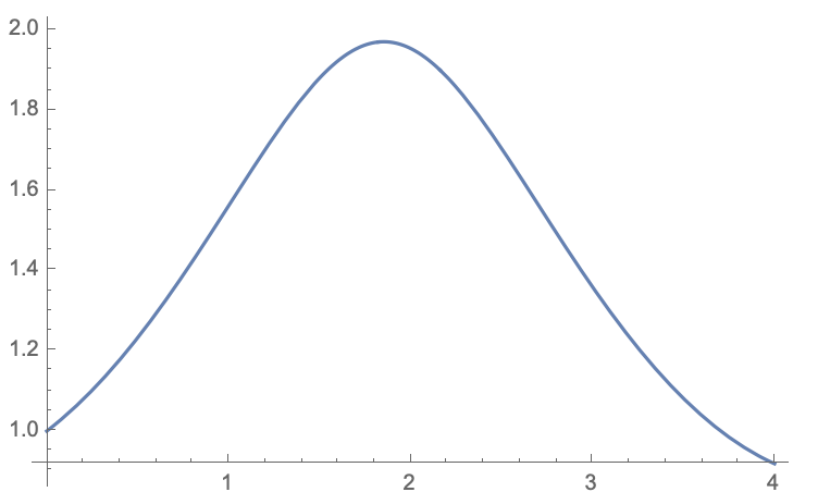
Plot[\[Theta][t] /. sol , {t, 0, 4}]
to get
The DAE solver in MMA is IDA (a portion of SUNDIALS developed by Lawrence Livermore National Labs)
If you apply the same tracing code that you posted to the "new" system with thPrime you see it also uses IDA because it becomes a DAE problem.
Select[Flatten[
  Trace[NDSolve[{\[Theta]'[t] == thPrime[t],
     eqN[[1]] /. \[Theta]'[t] -> thPrime[t], \[Theta][0] ==
      1}, {\[Theta][t], thPrime}, {t, 0, 4}],
   TraceInternal -> True]], ! FreeQ[#, Method | NDSolve`MethodData] &]
IDA will only be used for DAE systems so you cannot specify it for your original system.
Now to your real question. "Why is the DAE solver better at this problem?". First, the reason that the Sqrt fails is that the algorithm takes a step in theta near when the argument of the Sqrt goes to zero. The step in theta makes the derivative complex and the solver does not know what to do with that solution. In fact, it just keeps on integrating producing a complex result.
To see how changing to a DAE gets around this, let's solve your problem manually as a DAE. The first step is to add a new variable for theta'[t] and take a derivative of the algebraic constraint.
In[32]:= eqN[[1]] /. Derivative[1][\[Theta]][t] -> thPrime[t]

Out[32]= Sec[\[Theta][t]/
   2] (1 - Cos[\[Theta][t]] + 2 Cos[2 \[Theta][t]] +
    2 (1 + Cos[\[Theta][t]]) thPrime[t]^2) == 0

In[37]:= dalg = Simplify[
  D[eqN[[1]] /. Derivative[1][\[Theta]][t] -> thPrime[t], t] /.
   Derivative[1][\[Theta]][t] -> thPrime[t]]

Out[37]= Sec[\[Theta][t]/2]^2 thPrime[
   t] (5 Sin[\[Theta][t]/2] - 9 Sin[(3 \[Theta][t])/2] -
    6 Sin[(5 \[Theta][t])/2] -
    2 (Sin[\[Theta][t]/2] + Sin[(3 \[Theta][t])/2]) thPrime[t]^2 +
    32 Cos[\[Theta][t]/2]^3 Derivative[1][thPrime][t]) == 0
Solve this for thPrime'[t]:
In[38]:= dalgSolved = Solve[dalg,  thPrime'[t]]

Out[38]= {{Derivative[1][thPrime][t] ->
   1/32 Sec[\[Theta][t]/
     2]^2 (9 Sec[\[Theta][t]/2] Sin[(3 \[Theta][t])/2] +
      6 Sec[\[Theta][t]/2] Sin[(5 \[Theta][t])/2] - 5 Tan[\[Theta][t]/2] +
      2 Sec[\[Theta][t]/2] Sin[(3 \[Theta][t])/2] thPrime[t]^2 +
      2 Tan[\[Theta][t]/2] thPrime[t]^2)}}
Your new system of equations is
Equation 1
In[40]:= eq1 = First@First@ dalgSolved /. Rule -> Equal

Out[40]= Derivative[1][thPrime][t] ==
 1/32 Sec[\[Theta][t]/
   2]^2 (9 Sec[\[Theta][t]/2] Sin[(3 \[Theta][t])/2] +
    6 Sec[\[Theta][t]/2] Sin[(5 \[Theta][t])/2] - 5 Tan[\[Theta][t]/2] +
    2 Sec[\[Theta][t]/2] Sin[(3 \[Theta][t])/2] thPrime[t]^2 +
    2 Tan[\[Theta][t]/2] thPrime[t]^2)
Equation 2:
In[41]:= eq2 = \[Theta]'[t] == thPrime[t]

Out[41]= Derivative[1][\[Theta]][t] == thPrime[t]

In[42]:= eqN

Out[42]= {Sec[\[Theta][t]/
    2] (1 - Cos[\[Theta][t]] + 2 Cos[2 \[Theta][t]] +
     2 (1 + Cos[\[Theta][t]]) Derivative[1][\[Theta]][t]^2) ==
  0, \[Theta][0] == 1}
Find a starting value for thPrime[0]
thpStart =
 N[Solve[eqN[[1]] /.
     Derivative[1][\[Theta]][t] -> thPrime[t] /. \[Theta][t] -> 1,
   thPrime[t]]]
Now you can solve this ODE (no longer a DAE) but this new ODE has 2 variables instead of one and no Sqrt is ever taken.
In[55]:= manualDAESol =
 NDSolve[{eq1, eq2, \[Theta][0] == 1,
   thPrime[0] == thPrime[t] /. thpStart[[2]]}, {\[Theta][t],
   thPrime[t]}, {t, 0, 4}]
You get the same answer. The advantage of the manual approach is that you also get the second solution by changing thpStart[[2]] to the other solution. thpStart[[1]].
(And now you can see why there are two solutions when you solve it manually.)
I hope this answers your question.
Regards,
Neil


