Vanessa,
For ParametricPlot to work
$\phi$ cannot simultaneously be a dependent and independent variable. If you let
$x$ be the independent variable, you can obtain a ParametricPlot.
Manipulate[
Grid[
{{
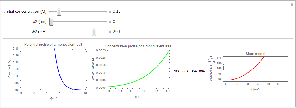
Plot[\[Phi][x, c0, \[Phi]2, x2], {x, 0, 10},
PlotRange -> {0, 0.3},
FrameLabel -> {Row[{Style["x", Italic], "[nm]"}],
Row[{Style["Potential", Italic], "(mV)"}]},
PlotLabel -> Row[{"Potential profile of a monovalent salt"}],
PlotStyle -> {Thick, Blue},
Frame -> True,
PerformanceGoal -> "Quality",
ImageSize -> 280
],
Plot[cf[x, c0, \[Phi]2, x2], {x, 0, 0.5},
PlotRange -> All,
FrameLabel -> {Row[{Style["x", Italic], "[nm]"}],
Row[{Style["Concentration", Italic], "(M)"}]},
PlotLabel -> Row[{"Concentration profile of a monovalent salt"}],
PlotStyle -> {Thick, Green},
Frame -> True,
PerformanceGoal -> "Quality",
ImageSize -> 280
],
ParametricPlot[{\[Phi][x, c0, \[Phi]2, x2],
cd[x, c0, \[Phi]2, x2]}, {x, 0, 10},
FrameLabel -> {Row[{Style["\[Phi]", Italic], "[mV]"}],
Row[{Style["Capacitance", Italic],
"(\!\(\*FractionBox[\(\[Micro]F\), SuperscriptBox[\(cm\), \
\(2\)]]\))"}]},
PlotLabel -> Row[{"Stern model"}],
PlotStyle -> {Thick, Red},
Frame -> True,
PerformanceGoal -> "Quality",
ImageSize -> 280
]
}}
],
{{c0, 0.15, "Initial concentration (M)"}, 0, 1,
Appearance -> "Labeled"},
{{x2, 0, "x2 (nm)"}, 0, 2, Appearance -> "Labeled"},
{{\[Phi]2, 200, "\[Phi]2 (mV)"}, 0, 250, Appearance -> "Labeled"},
Initialization :> (
z = 1;
T = 300;
\[Epsilon]0 = 8.854*10^-12;
\[Epsilon] = 80;
R = 8.314;
F = 96485.33;
xmax = 20;
\[Kappa][
c0_] := (((2*(c0*1000)*F^2)/(\[Epsilon]*\[Epsilon]0*R*T))^(
1/2)*10^-9);
\[Phi][x_, c0_, \[Phi]2_, x2_] := \[Phi]2*
Exp[-\[Kappa][c0]*(x - x2)];
cf[x_, c0_, \[Phi]2_, x2_] :=
c0*Exp[-z*F*\[Phi][x, c0, \[Phi]2, x2]/(1000*R*T)];
cd[x_, c0_, \[Phi]2_,
x2_] := ((x2*10^-11)/(\[Epsilon]*\[Epsilon]0) + (
1*10^-11)/(\[Epsilon]*\[Epsilon]0*\[Kappa][c0]*
Cosh[(z*F*\[Phi][x, c0, \[Phi]2, x2])/(2*1000*R*T)]))^-1;
)
]