NOTE: Download Full Article as a Notebook from the Attachment Below
Interphase mass transfer operations such as gas absorption or liquid-liquid extraction pose a modeling challenge because the molar species concentration can jump between 2 states at the interface as shown below (from here). 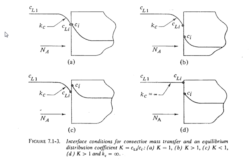 I wanted to see if I could create a Finite Element Method (FEM) model of jump conditions in the Wolfram Language. I found the results to be reasonable, aesthetically pleasing, and somewhat mesmerizing. The remainder of this post documents my workflow for those that might be interested. I have attached a notebook to reproduce the results.
Preamble on analytical solutions to PDE's
There seems to be quite a few posts where people are trying to find the analytical solution to a system of PDE's. Generally, closed formed analytical solutions only exist in rare-highly symmetric cases. Let us consider the heat equation below.
$$\frac{\partial T}{\partial t}=\alpha \frac{\partial^2 T}{\partial x^2}$$
For the case of a semi-infinite bar subjected to a unit step change in temperature at $x=0$, Mathematica's DSolve[] handles this readily.
u[x, t] /.
 First@DSolve[{ D[u[x, t], t] == alpha D[u[x, t], {x, 2}],
    u[x, 0] == 0, u[0, t] == UnitStep[t]}, u[x, t], {x, t},
   Assumptions -> alpha > 0 && 0 < x]
(*Erfc[x/(2*Sqrt[alpha]*Sqrt[t])]*)
So far so good. Now, let us break symmetry by making it a finite bar of length $l$ (See Documentation).
heqn = D[u[x, t], t] == alpha D[u[x, t], {x, 2}];
bc = {u[0, t] == 1, u[l, t] == 0};
ic = u[x, 0] == 0;
sol = DSolve[{heqn, bc, ic}, u[x, t], {x, t}]
(*{{u[x, t] -> 1 - x/l - (2*Inactive[Sum][Sin[(Pi*x*K[1])/l]/(E^((alpha*Pi^2*t*K[1]^2)/l^2)*
         K[1]), {K[1], 1, Infinity}])/Pi}}*)
This little change going from a semi-infinite to finite domain has turned the solution into an unwieldy infinite sum. We should expect that it will only go down hill from here if we add additional complexity to the equation or system of equations. My advice is to abandon the search for an analytical solution quickly because it will likely take great effort and will be unlikely to yield a result. Instead, focus efforts on more productive avenues such as dimensional analysis and numerical solutions.
Introduction
"All models are wrong, some are useful." -- George E. P. Box "However, many systems are highly complex, so that valid mathematical models of them are themselves complex, precluding any possibility of an analytical solution. In this case, the model must be studied by means of simulation, i.e. , numerically exercising the model for the inputs in question to see how they affect the output measures of performance." -- Dr. Averill Law, Simulation Modeling and Analysis
I find the quotes above help me overcome inertia when starting a modeling and simulation project. Create your wrong model. Calibrate how wrong it is versus a known standard. If it is not too bad, put the model through its paces.
One thing that I appreciate about the Wolfram Language is that I can document a modeling workflow development process from beginning to end in a single notebook. The typical model workflow development process includes:
- A sketch of the system of interest.
- Equations.
- Initial development.
- Simplification.
- Non-dimensionalization for better scaling and reducing parameter space.
- Mathematica implementation.
- Mesh
- NDSolve set-up
- Post-process results
- Verification/Validation
Mathematica notebooks tend to age well. I routinely resurrect notebooks that are over a decade old and they generally still work.
Absorption
I did a quick Google search on absorption and came across this figure describing gas absorption in an open access article by Danish et al.
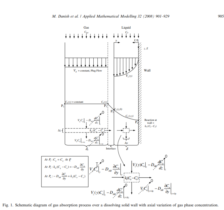
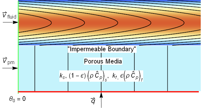
This image looked very similar to an image that I produced in a related post to the Wolfram community regarding porous media energy transport.
The systems look so similar, that we ought to be able to reuse much of the modeling. An area of concern would be for gas absorption where the ratio of the gas diffusion coefficient to liquid diffusion coefficient can exceed 4 orders of magnitude. Such differences often can cause instability in numerical approaches.
Modeling
System description
For clarity, I always like to begin with a system description. Typically, absorption processes utilize gravity to create a thin liquid film to contact the gas. To reuse the modeling that we did for porous media, we will assume that gravity is in the positive $x$ direction leading us to the image below.
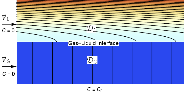
We will assume that the liquid film is a uniform thickness and is laminar (note that for gas liquid contact the liquid velocity is fastest at the interface leading to the parabolic profile shown). We will assume that the gas has a uniform velocity. Further, we will assume that the incoming concentrations of the absorbing species are zero and we will impose a concentration of $C=C_0$ at the lower boundary.
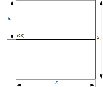
The basic dimensions of the box are shown below. For simplicity, we will make the height and length unit dimensions and set $R$ to be $\frac{1}{2}$.
Balance equations
Dilute species balance
For the purposes of this exercise, we will consider the system to be dilute such that diffusion does not affect the overall flow velocities. Within a single phase, the molar balance of concentration is given by equation (1). We will assume steady-state operation with no reactions so that we can eliminate the red terms.
$${\color{Red}{\frac{{\partial {C}}}{{\partial t}}}} + \mathbf{v} \cdot \nabla C - \nabla \cdot \mathcal{D} \nabla C - {\color{Red}{r^{'''}}} = 0 \qquad (1)$$
Species balance in each phase
For convenience, I will denote the phases by a subscript G and L for gas and liquid with the understanding that these equations could also apply to a liquid-liquid extraction problem. This leads to the following concentration balance equations for the liquid and gas phases.
$$\begin{gathered} \begin{matrix} \mathbf{v}_L \cdot \nabla C_L + \nabla \cdot \left(-\mathcal{D}_L \nabla C_L\right) = 0 & x,y\in \Omega_L & (2*) \\ \mathbf{v}_G \cdot \nabla C_G + \nabla \cdot \left(-\mathcal{D}_G \nabla C_G\right) = 0 & x,y\in \Omega_G & (3*) \\ \end{matrix} \end{gathered}$$
Or in Laplacian form
$$\begin{gathered} \begin{matrix} \mathbf{v}_L \cdot \nabla C_L -\mathcal{D}_L \nabla^2 C_L = 0 & x,y\in \Omega_L & (2*) \\ \mathbf{v}_G \cdot \nabla C_G -\mathcal{D}_G \nabla^2 C_G = 0 & x,y\in \Omega_G & (3*) \\ \end{matrix} \end{gathered}$$
Creating a No-Flux Boundary Condition at the Interface
To prevent the gas species diffusing into the liquid layer and vice versa, I will set the velocities to zero and the diffusion coefficients to a very small value in the other phase. From a visualization standpoint, it will appear that the gas species has diffused into the liquid layer and vice versa, but the flux is effectively zero. To clean up the visualization, we will define plot ranges by gas, interphase, and liquid regions.
Species balance including a thin interphase region
We will define a thin Interphase region between the 2 phases that will allow us to couple the phases in the interphase region via a source term creating the jump discontinuity in concentration as shown in the figure below.
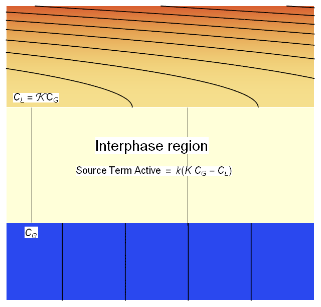
We will modify (2*) and (3*) with the coupling source term as shown below.
$$\begin{gathered} \begin{matrix} \mathbf{v}_L \cdot \nabla C_L -\mathcal{D}_L \nabla^2 C_L - \sigma\left(\Omega \right )k\left(K C_G-C_L \right ) = 0 & x,y\in \Omega & (2) \\ \mathbf{v}_G \cdot \nabla C_G -\mathcal{D}_G \nabla^2 C_G + \sigma\left(\Omega \right )k\left(K C_G-C_L \right ) = 0 & x,y\in \Omega & (3) \\ \end{matrix} \end{gathered}$$
Where $K$ is a vapor-liquid equilibrium constant, $k$ is in interphase mass transfer coefficient (we will make this large because we want a fast approach to equilibrium), and $\sigma$ is a switch that turns on (=1) in the interface region and 0 otherwise.
Dimensional analysis
We will multiply equations (2) and (3) by $\frac{{R^2}}{C_0 \mathcal{D}_G}$ to obtain their non-dimensionalized forms (4) and (5).
$$\begin{gathered} \begin{matrix} C_0\left (\frac{\mathbf{v}_L}{R} \cdot \nabla^* C_{L}^{*} -\frac{\mathcal{D}_L}{R^2} \nabla^{*2} C_{L}^{*} - \sigma\left(\Omega \right )k\left(K C_{G}^{*}-C_{L}^{*} \right ) \right ) = 0\left\| {\frac{{R^2}}{C_0 \mathcal{D}_G}} \right. \\ C_0\left (\frac{\mathbf{v}_G}{R} \cdot \nabla^* C_{G}^{*} -\frac{\mathcal{D}_G}{R^2} \nabla^{*2} C_{G}^{*} + \sigma\left(\Omega \right )k\left(K C_{G}^{*}-C_{L}^{*} \right ) \right ) = 0\left\| {\frac{{R^2}}{C_0 \mathcal{D}_G}} \right. \\ \end{matrix} \end{gathered}$$
$$\begin{gathered} \begin{matrix} \frac{\mathcal{D}_L}{\mathcal{D}_G} \frac{R\mathbf{v}_L}{\mathcal{D}_L} \cdot \nabla^* C_{L}^{*} -\delta \nabla^{*2} C_{L}^{*} - \sigma\left(\Omega \right )\kappa\left(K C_{G}^{*}-C_{L}^{*} \right ) = 0 \\ \frac{R\mathbf{v}_G}{\mathcal{D}_G} \cdot \nabla^* C_{G}^{*} - \nabla^{*2} C_{G}^{*} + \sigma\left(\Omega \right )\kappa\left(K C_{G}^{*}-C_{L}^{*} \right ) = 0\\ \end{matrix} \end{gathered}$$
$$\begin{gathered} \begin{matrix} \delta{Pe}_L\mathbf{v}_{L}^* \cdot \nabla^* C_{L}^{*} -\delta \nabla^{*2} C_{L}^{*} - \sigma\left(\Omega \right )\kappa\left(K C_{G}^{*}-C_{L}^{*} \right ) = 0 & (4) \\ {Pe}_G\mathbf{v}_{G}^* \cdot \nabla^* C_{G}^{*} - \nabla^{*2} C_{G}^{*} + \sigma\left(\Omega \right )\kappa\left(K C_{G}^{*}-C_{L}^{*} \right ) = 0 &(5)\\ \end{matrix} \end{gathered}$$
Where
$$\delta=\frac{\mathcal{D}_L}{\mathcal{D}_G}$$ $$Pe_L=\frac{R\mathbf{v}_L}{\mathcal{D}_L}$$ $$Pe_G=\frac{R\mathbf{v}_G}{\mathcal{D}_G}$$
With a good dimensionless model in place, we can start with our Wolfram Language implementation.
Wolfram Language Implementation
Mesh creation
We start by loading the FEM package.
Needs["NDSolve`FEM`"]
When I started this effort, I considered co-current flow only. I realized that converting the model to counter-current flow was a simple matter of changing boundary markers. I wrapped the process up in a module that returns an association whose parameters can be used to set up an NDSolve solution. In the counter-current case, I changed the bottom boundary to a wall and the gas inlet concentration to 1.
makeMesh[h_, l_, rat_, gf_, cf_] :=
 Module[{bR, tp, bt, lf, rt, th, interfacel, interfaceg, buf, bnds,
   rgs, crds, lelms, boundaryMarker, bcEle, bmsh, liquidCenter,
   liquidReg, interfaceCenter, interfaceReg, gasCenter, gasReg,
   meshRegs, msh, mDic},
  (* Domain Dimensions *)
  bR = rat h;
  tp = bR;
  bt = bR - h;
  lf = 0;
  rt = l;
  th = h/gf;
  interfacel = 0;
  interfaceg = interfacel - th;
  buf = 2.5 th;

  (* Use associations for clearer assignment later *)
  bnds = <|liquidinlet -> 1, gasinlet -> 2, bottom -> 3|>;
  rgs = <|gas -> 10, liquid -> 20, interface -> 15|>;

  (* Meshing Definitions *)
  (* Coordinates *)
  crds = {{lf, bt}(*1*), {rt, bt}(*2*), {rt, tp}(*3*), {lf,
     tp}(*4*), {lf, interfacel}(*5*), {rt, interfacel}(*6*), {lf,
     interfaceg}(*7*), {rt, interfaceg}(*8*)};

  (* Edges *)
  lelms = {{1, 7}, {7, 5}, {5, 4}, {1, 2},
           {2, 8}, {8, 6}, {6, 3}, {3, 4},
           {5, 6}, {7, 8}};

  (* Conditional Boundary Markers depending on configuration *)
  boundaryMarker := {bnds[gasinlet], bnds[liquidinlet],
     bnds[liquidinlet], bnds[bottom], 4, 4, 4, 4, 4, 4} /; cf == "Co";
  boundaryMarker := {4, 4, bnds[liquidinlet], bnds[bottom],
     bnds[gasinlet], 4, 4, 4, 4, 4} /; cf == "Counter";

  (* Create Boundary Mesh *)
  bcEle = {LineElement[lelms, boundaryMarker]};
  bmsh = ToBoundaryMesh["Coordinates" -> crds,
    "BoundaryElements" -> bcEle];

  (* 2D Regions *)
  (* Identify Center Points of Different Material Regions *)
  liquidCenter = {(lf + rt)/2, (tp + interfacel)/2};
  liquidReg = {liquidCenter, rgs[liquid], 0.0005};
  interfaceCenter = {(lf + rt)/2, (interfacel + interfaceg)/2};
  interfaceReg = {interfaceCenter, rgs[interface], 0.5*0.000005};
  gasCenter = {(lf + rt)/2, (bt + interfaceg)/2};
  gasReg = {gasCenter, rgs[gas], 0.0005};
  meshRegs = {liquidReg, interfaceReg, gasReg};

  msh = ToElementMesh[bmsh, "RegionMarker" -> meshRegs,
    MeshRefinementFunction -> Function[{vertices, area},
      Block[{x, y},
       {x, y} = Mean[vertices];
       If[
        (y > interfaceCenter[[2]] - buf &&
            y < interfaceCenter[[2]] + buf)  ||
         (y < bt + 1.5 buf &&
            x < lf + 1.5 buf)
        , area > 0.0000125, area > 0.01
        ]
       ]
      ]
    ];

  mDic = <|
    height -> h,
    length -> l,
    ratio -> rat,
    gapfactor -> gf,
    r -> bR,
    top -> tp,
    bot -> bt,
    left -> lf,
    right -> rt,
    intl -> interfacel,
    intg -> interfaceg,
    intcx -> interfaceCenter[[1]],
    intcy -> interfaceCenter[[2]],
    buffer -> buf,
    mesh -> msh,
    bmesh -> bmsh,
    bounds -> bnds,
    regs -> rgs,
    cfg -> cf
    |>;
  mDic]

Options[meshfn] = {height -> 1, length -> 1, ratio -> 0.5,
   gapfactor -> 100, config -> "Co"};
meshfn[OptionsPattern[]] :=
 makeMesh[OptionValue[height], OptionValue[length],
  OptionValue[ratio], OptionValue[gapfactor], OptionValue[config]]
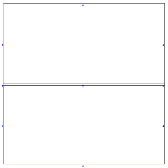
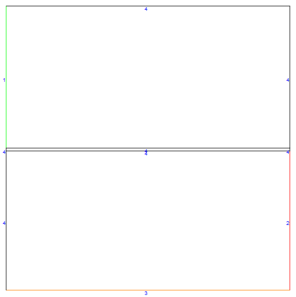
We can create a mesh instance of a co-current flow case by invoking the meshfn[]. I will color the liquid inlet $\color{Green}{Green}$, the gas inlet $\color{Red}{Red}$ and the bottom boundary $\color{Orange}{Orange}$ (the rest of the boundaries are default).
mDicCo = meshfn[config -> "Co"];
mDicCo[bmesh][
 "Wireframe"["MeshElementMarkerStyle" -> Blue,
  "MeshElementStyle" -> {Green, Red, Orange, Black},
  ImageSize -> Large]]
By setting the optional config parameter to "Counter", we can easily generate a counter-current case as shown below (note how the gas inlet shifted to the right side.
mDic = meshfn[config -> "Counter"];
mDic[bmesh][
 "Wireframe"["MeshElementMarkerStyle" -> Blue,
  "MeshElementStyle" -> {Green, Red, Orange, Black},
  ImageSize -> Large]]
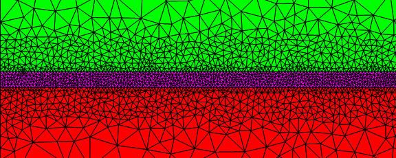
For the co-current case, the bottom wall and the gas inlet have inconsistent Dirichlet conditions. To reduce the effect, I refined the mesh in the lower left corner as shown below.
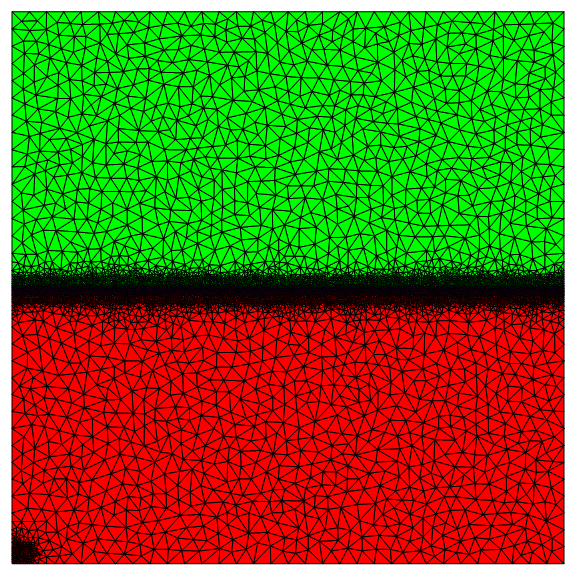
I also meshed the interface region finely.
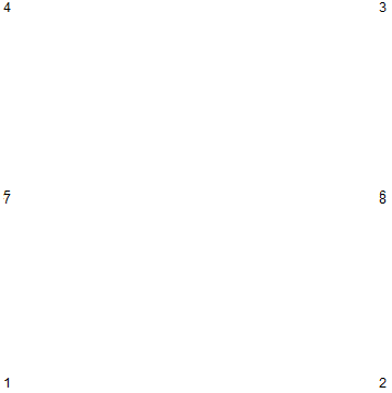
Sometimes it can get confusing to setup alternative boundaries. To visualize the coordinate IDs, you could use something like:
With[{pts = mDic[bmesh]["Coordinates"]},
 Graphics[{Opacity[1], Black,
   GraphicsComplex[pts,
    Text[Style[ToString[#], Background -> White, 12], #] & /@
     Range[Length[pts]]]}]]
Solving and Visualization
I have created a module that will solve and visualize depending on the mesh type (co-flow or counter-flow). Hopefully, it is well enough commented that further discussion is not needed.
model[md_, kequil_, d_, pel_, peg_, title_] :=
  Module[{n, pecletgas, por, vl, vg, fac, facg, coefl, coefg,
    dcliquidinletliquid, dcliquidinletgas, dcinletgas,
    dcgasinletliquid, dcgasinletgas, dcbottomliquid, dcbottomgas,
    eqnliquid, eqngas, eqns, ifun, pltl, pltint, pltg, pltarr, sz,
    grid, lf, rt, tp, bt, interfaceg, interfacel, interfaceCenterY,
    plrng, arrequil, arrdiff, arrgas,
    arrliq},
   (*localize Mesh Dict Values*)lf = md[left];
   rt = md[right];
   tp = md[top];
   bt = md[bot];
   interfaceg = md[intg];
   interfacel = md[intl];
   interfaceCenterY = md[intcy];
   (*Must swtich gas flow direction for counter-flow*)
   pecletgas = If[md[cfg] == "Co", peg, -peg];
   (*Dimensionless Mass Transfer Coefficient in Interphase Region*)
   n = 10000;
   (*"Porosity" to weight concentration in interphase*)
   por[y_, intg_, intl_] := (y - intg)/(intl - intg);
   (*Region Dependent Properties with Piecewise \
Functions*)(*velocity*)(*Liquid parabolic profile*)
   vl = Evaluate[
     Piecewise[{{{pel d (1 - (y/md[r])^2), 0},
        ElementMarker == md[regs][liquid]}, {{pecletgas, 0},
        ElementMarker == md[regs][gas]}, {{0, 0}, True}}]];
   (*Gas Uniform Velocity*)
   vg = Evaluate[
     Piecewise[{{{pecletgas, 0},
        ElementMarker == md[regs][gas]}, {{pel d (1 - (y/md[r])^2),
         0}, ElementMarker == md[regs][liquid]}, {{0, 0}, True}}]];
   (*fac switches on mass transfer coefficient in interphase*)
   fac = Evaluate[If[ElementMarker == md[regs][interface], n, 0]];
   (*diffusion coefficients*)(*Liquid*)
   coefl = Evaluate[
     Piecewise[{{d, ElementMarker == md[regs][liquid]}, {1,
        ElementMarker == md[regs][interface]}, {d/1000000,
        True} (*Effectively No Flux at Interface*)}]];
   (*Gas*)coefg =
    Evaluate[
     Piecewise[{{1, ElementMarker == md[regs][gas]}, {1,
        ElementMarker == md[regs][interface]}, {d/1000000,
        True} (*Effectively No Flux at Interface*)}]];
   (*Dirichlet Conditions for Liquid at Inlets*)
   dcliquidinletliquid =
    DirichletCondition[cl[x, y] == 0,
     ElementMarker == md[bounds][liquidinlet]];
   dcliquidinletgas =
    DirichletCondition[cg[x, y] == 0,
     ElementMarker == md[bounds][liquidinlet]];
   dcgasinletliquid =
    DirichletCondition[cl[x, y] == 0,
     ElementMarker == md[bounds][gasinlet]];
   (*Conditional BCs for gas dependent on configuration*)
   dcgasinletgas :=
    DirichletCondition[cg[x, y] == 0,
      ElementMarker == md[bounds][gasinlet]] /; md[cfg] == "Co";
   dcgasinletgas :=
    DirichletCondition[cg[x, y] == 1,
      ElementMarker == md[bounds][gasinlet]] /; md[cfg] == "Counter";
   (*Dirichlet Conditions for the Bottom Wall*)
   dcbottomliquid =
    DirichletCondition[cl[x, y] == 0,
     ElementMarker == md[bounds][bottom]];
   dcbottomgas =
    DirichletCondition[cg[x, y] == 1,
     ElementMarker == md[bounds][bottom]];
   (*Balance Equations for Gas and Liquid Concentrations*)
   eqnliquid =
    vl.Inactive[Grad][cl[x, y], {x, y}] -
      coefl Inactive[Laplacian][cl[x, y], {x, y}] -
      fac (kequil cg[x, y] - cl[x, y]) == 0;
   eqngas =
    vg.Inactive[Grad][cg[x, y], {x, y}] -
      coefg Inactive[Laplacian][cg[x, y], {x, y}] +
      fac (kequil cg[x, y] - cl[x, y]) == 0;
   (*Equations to be solved depending on configuration*)
   eqns := {eqnliquid, eqngas, dcliquidinletliquid, dcliquidinletgas,
      dcgasinletliquid, dcgasinletgas, dcbottomliquid, dcbottomgas} /;
      md[cfg] == "Co";
   eqns := {eqnliquid, eqngas, dcliquidinletliquid, dcliquidinletgas,
      dcgasinletliquid, dcgasinletgas} /; md[cfg] == "Counter";
   (*Solve the PDE*)
   ifun = NDSolveValue[eqns, {cl, cg}, {x, y} \[Element] md[mesh]];
   (*Visualizations*)(*Create Arrows to represent magnitude of \
dimensionless groups*)(*Equilibrium Arrow*)
   arrequil = {CapForm["Square"], Red, Arrowheads[0.03],
     Arrow[Tube[{{1 - 0.0125, 0.025, 1}, {1 - 0.0125, 0.025, kequil}},
        0.005], -0.03]};
   (*Diffusion Arrow*)
   arrdiff = {Darker[Green, 1/2],
     Arrowheads[0.03, Appearance -> "Flat"],
     Arrow[Tube[{{-0.025, 0.0, 0.0 .025}, {-0.025,
         0.5 (1 + Log10[d]/4), 0.025}}, 0.005], -0.03]};
   (*Liquid Peclet Arrow*)
   arrliq = {Blue, Dashed, Arrowheads[1.5 0.03],
     Arrow[Tube[{{0.0, mDic[top] + 0.025, 0.035}, {pel/50,
         mDic[top] + 0.025, 0.035}}, 1.5 0.005], -0.03 1.5]};
   (*Conditional Gas Peclet Arrow*)
   arrgas := {Black, Dashed, Arrowheads[1.5 0.03],
      Arrow[Tube[{{0.0, mDic[bot], 1.035}, {peg/50, mDic[bot],
          1.035}}, 1.5 0.005], -0.03 1.5]} /; md[cfg] == "Co";
   arrgas := {Black, Dashed, Arrowheads[1.5 0.03],
      Arrow[Tube[{{mDic[right], mDic[bot],
          1.035}, {mDic[right] - peg/50, mDic[bot], 1.035}},
        1.5 0.005], -0.03 1.5]} /; md[cfg] == "Counter";
   (*Set up plots*)(*Common plot options*)
   plrng = {{lf, rt}, {bt, tp}, {0, 1}};
   SetOptions[Plot3D, PlotRange -> plrng, PlotPoints -> {200, 200},
    ColorFunction ->
     Function[{x, y, z}, Directive[ColorData["DarkBands"][z]]],
    ColorFunctionScaling -> False, MeshFunctions -> {#3 &},
    Mesh -> 18, AxesLabel -> Automatic, ImageSize -> Large];
   (*Liquid Plot*)
   pltl = Plot3D[ifun[[1]][x, y], {x, lf, rt}, {y, interfacel, tp},
     MeshStyle -> {Black, Thick}];
   (*Interface region Plot*)
   pltint =
    Plot3D[ifun[[2]][x, y] (1 - por[y, interfaceg, interfacel]) +
      por[y, interfaceg, interfacel] ifun[[1]][x, y], {x, lf, rt}, {y,
       interfaceg, interfacel},
     MeshStyle -> {DotDashed, Black, Thick}];
   (*Gas Plot*)
   pltg = Plot3D[ifun[[2]][x, y], {x, lf, rt}, {y, bt, interfaceg},
     MeshStyle -> {Dashed, Black, Thick}];
   (*Grid Plot*)sz = 300;
   grid =
    Grid[{{Show[{pltl, pltint, pltg},
        ViewProjection -> "Orthographic", ViewPoint -> Front,
        ImageSize -> sz, Background -> RGBColor[0.84`, 0.92`, 1.`],
        Boxed -> False],
       Show[{pltl, pltint, pltg}, ViewProjection -> "Orthographic",
        ViewPoint -> Left, ImageSize -> sz,
        Background -> RGBColor[0.84`, 0.92`, 1.`],
        Boxed -> False]}, {Show[{pltl, pltint, pltg},
        ViewProjection -> "Orthographic", ViewPoint -> Top,
        ImageSize -> sz, Background -> RGBColor[0.84`, 0.92`, 1.`],
        Boxed -> False],
       Show[{pltl, pltint, pltg}, ViewProjection -> "Perspective",
        ViewPoint -> {Above, Left, Back}, ImageSize -> sz,
        Background -> RGBColor[0.84`, 0.92`, 1.`], Boxed -> False]}},
     Dividers -> Center];
   (*Reset Plot Options to Default*)
   SetOptions[Plot3D, PlotStyle -> Automatic];
   pltarr =
    Grid[{{Text[Style[title, Blue, Italic, 24]]}, {Style[
        StringForm[
         "\!\(\*SubscriptBox[\(K\), \(C\)]\)=``, \[Delta]=``, \
\!\(\*SubscriptBox[\(Pe\), \(L\)]\)=``, and \
\!\(\*SubscriptBox[\(Pe\), \(G\)]\)=``",
         NumberForm[kequil, {3, 2}, NumberPadding -> {" ", "0"}],
         NumberForm[d, {5, 4}, NumberPadding -> {" ", "0"}],
         NumberForm[pel, {2, 1}, NumberPadding -> {" ", "0"}],
         NumberForm[peg, {2, 1}, NumberPadding -> {" ", "0"}]],
        18]}, {Show[{pltl, pltint, pltg,
         Graphics3D[{arrequil, arrdiff, arrliq, arrgas}](*,arrequil,
         arrdiff,arrliq,arrgas*)}, ViewProjection -> "Perspective",
        ViewPoint -> {Above, Left, Back}, ImageSize -> 640,
        Background -> RGBColor[0.84`, 0.92`, 1.`], Boxed -> False,
        PlotRange -> {{md[left] - 0.05, md[right]}, {md[bot],
           md[top] + 0.05}, {0, 1 + 0.1}}]}}];
   (*Return values*){ifun, {pltl, pltint, pltg}, pltarr, grid}];

Options[modelfn] = {md -> mDic, k -> 0.5, dratio -> 1, pel -> 50,
   peg -> 50, title -> "Test"};
modelfn[OptionsPattern[]] :=
 model[OptionValue[md], OptionValue[k], OptionValue[dratio],
  OptionValue[pel], OptionValue[peg], OptionValue[title]]
Testing of Meshing and Solving Modules
Now, that we wrapped our meshing and solving work flow into modules, I will demonstrate how to create an instance of a simulation.
(* Create a Co-Flow Mesh *)
mDic = meshfn[config -> "Co"];
(* Simulate and return results *)
res = modelfn[md -> mDic, k -> 0.5, dratio -> 0.1, pel -> 10,
   peg -> 5, title -> "Co-Flow"];
To visualize a 3D plot with arrows representing the magnitude of dimensionless parameters, we access the third part of the results list.
res[[3]]
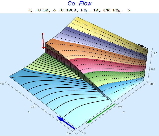
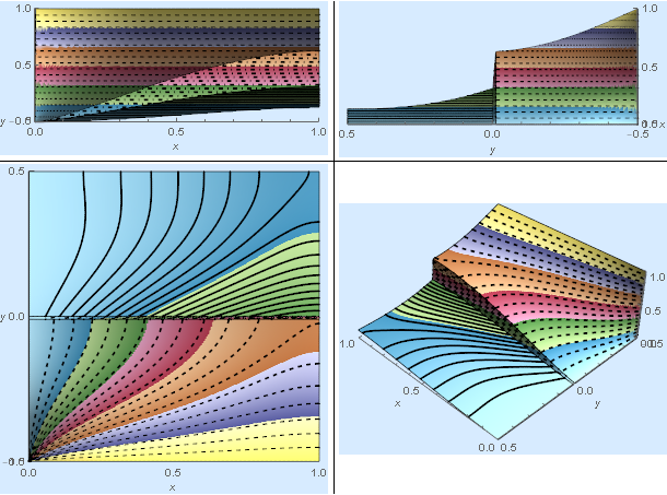
The solid lines, dashed lines, and dashed-dotted lines represent contours of species concentration in the liquid, gas, and interphase regions, respectively. The $\color{Red}{Red}$ arrow is proportional to (1-K), the $\color{Green}{Green}$ arrow is proportional to the log of the diffusion ratio $\delta$, the $\color{Blue}{Blue}$ arrow is proportional to $Pe_L$, and the $\color{Black}{Black}$ arrow is proportional to $Pe_G$. Multiple views are contained in part 4 of the results list.
res[[4]]
Validation (Comparison to another code)
Before continuing, it is always good practice to validate your model versus experiment or at least another code. The other code supports a partition conditions for the concentration jump so that I do not need to create an interface layer. The results are shown below:
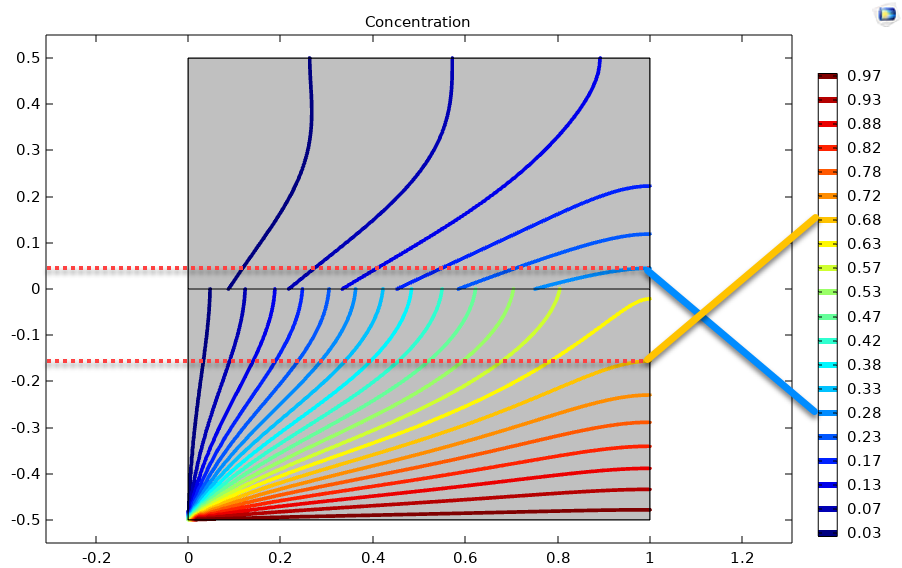
The contour plots look very similar to the image in the lower left corner of the grid plot. To be more quantitative, I have highlighted contours at approximately y=-0.15 and y=0.05 in the gas and liquid layers at x=1 corresponding to concentrations of 0.68 and 0.28, respectively. The first part of the results list returns an interpolation function of the liquid and gas species. We can see that we are within a percent of the other code, which is reasonable given that the interface layer is about 1% of the domain. This check gives me good confidence that my model is not too wrong and that I can start to make it useful (i.e., exercising the model by changing parameters).
res[[1]][[2]][1, -0.15] (*0.6769985984321076`*)
res[[1]][[1]][1, 0.05] (* 0.27374616012596314`*)
Generating Animations
I like to animate. For me, animations are the best way to demonstrate how a system evolves as a function of time or parameter changes. We can export an animated gif file to study the effects of dimensionless parameter changes for both flow configurations as shown in the following code. It will take about 30 minutes per animation and about 5 GB of RAM. Undoubtedly, this code could be optimized for speed and memory usage, but you still can create a dozen animations while you sleep.
SetDirectory[NotebookDirectory[]];

f = ((#1 - #2)/(#3 - #2)) &; (* Scale for progress bar *)

mDic = meshfn[config -> "Counter"]; (* Create Mesh Instance *)

Export["CounterFlow.gif",
 Monitor[
  Table[
   modelfn[md -> mDic, k -> kc, dratio -> 1, pel -> 0, peg -> 0,
     title -> "Counter-Flow"][[3]], {kc, 1, 0.01, -0.01}
    ],
  Grid[
    {{"Total progress:",
     ProgressIndicator[
      Dynamic[f[kc, 1,
        0.01, -0.01]]]}, {"\!\(\*SubscriptBox[\(K\), \(C\)]\)=", \
{Dynamic@kc}}}]
    ],
 "AnimationRepetitions" -> \[Infinity]]
Examples
I combined the co- (left) and counter-current (right) gif animations for several cases below. Péclet numbers approaching 100 start to look uninteresting visually (all the action is very close to the interface). This should inform the user that perhaps another model is in order with new assumptions to study the small-scale behavior near the interface.
Changing the Equilibrium Constant @ No Flow

As the equilibrium constant, $K$, reduces, the jump condition increases.
Changing the Diffusion Ratio $\delta$ @ No Flow
As the liquid-gas diffusion ratio, $\delta$, decreases, the concentration in the gas layer increases. We also see that the solution does not change much for $\delta<0.01$.
Changing $Pe_L$ @ No Gas Flow
As $Pe_L$ increases, the concentration gradient increases at the interface.
Changing $Pe_G$ @ No Liquid Flow

As $Pe_G$ increases, we see the concentration in the liquid layer decrease for co-flow and increase for counter-current flow. This should make sense since the inlet concentration for co-flow is 0 and 1 for counter-current flow.
Changing the Diffusion Ratio $\delta$ @ Middle Conditions
Again, we do not see much change for $\delta<0.01$. One may have noticed that the concentration in the liquid layer goes up as the diffusion coefficient ratio goes down, which may, at first, seem counterintuitive. The reason for this behavior is that the dimensionless velocity in the liquid layer depends on both $Pe_L$ and $\delta$ so it decreases with decreasing $\delta$.
Summary
- Constructed an FEM model in the Wolfram Language to study concentration jump conditions in interphase mass transfer.
- Results compare favorably to another code designed to handle jump conditions.
- Showed several examples of the effect of dimensionless parameter changes on two model flow configurations.
- Notebook provided.
 Attachments:


