I recently finished a major overhaul of my Bayesian inference package on Github:

https://github.com/ssmit1986/BayesianInference

and wanted to give a small overview of what it can do. If you're interested, the repository has a notebook with other examples to browse through. As an example, let's do some regression on financial data:

<< BayesianInference`;
data = FinancialData["AS:ASML", {Today - Quantity[3, "Months"], Today}];
DateListPlot[data]

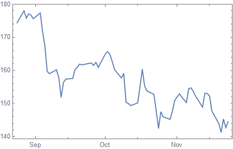
Preparation of the data:

data = TimeSeriesRescale[data, {0, Length[data] - 1}];
{start, ts} = TakeDrop[data, 1];
start = start[[1, 2]];
ts = TimeSeries[ts];

We will try to model the data with a GeometricBrownianMotionProcess (GBP):

process = GeometricBrownianMotionProcess[mu, Exp[logsigma], start]; (* using Exp[logsigma] makes it easier to search for sigma values over a large range of values *)

The goal of what follows below is to find values for mu and sigma that can fit the data well. However, we want to do this the Bayesian way and find a proper probability distribution over these two parameters that tells us precisely how much we can know about mu and sigma.

My package uses the function defineInferenceProblem to specify all of the relevant inputs for the problem. You can check the types of recognised input with defineInferenceProblem[]:

In[77]:= defineInferenceProblem[]
Out[77]= {Data,Parameters, IndependentVariables, LogLikelihoodFunction, LogPriorPDFFunction, GeneratingDistribution, PriorDistribution, PriorPDF}

You don't need to specify everything in this list: only whatever is necessary to compute the loglikelihood function and the logPDF of the prior (it's important to work with these log functions to avoid numerical rounding errors). For example, this is how we can define the inference problem for the GBP regression:

obj = defineInferenceProblem[
  "Data" -> ts,
  "GeneratingDistribution" -> process[t],
  "Parameters" -> {{mu, -\[Infinity], \[Infinity]}, {logsigma, -\[Infinity], \[Infinity]}},
  "IndependentVariables" -> {t}, 
  "PriorDistribution" -> {NormalDistribution[0, 10], NormalDistribution[0, 10]}
  ]

This is a somewhat naive way to do the regression, because it models the data points as independent realizations of a log normal distribution rather than as sequentially dependent realizations of the GBP. In the example code on Github there is an explanation on how to model the GBP properly.

The returned object is basically an Association that keeps all of the relevant data together. To inference the posterior distribution of mu and sigma, we use the nested sampling algorithm by John Skilling. This algorithm will produce (weighted) samples from the posterior and compute the evidence integral (which measures the quality of the fit). I implemented a normal version and a parallel version. It is called like so:

result = parallelNestedSampling[obj];

Visualise the samples with a bubble chart (where the sizes are the weights):

posteriorBubbleChart[takePosteriorFraction[result, 0.99], {mu, logsigma}]

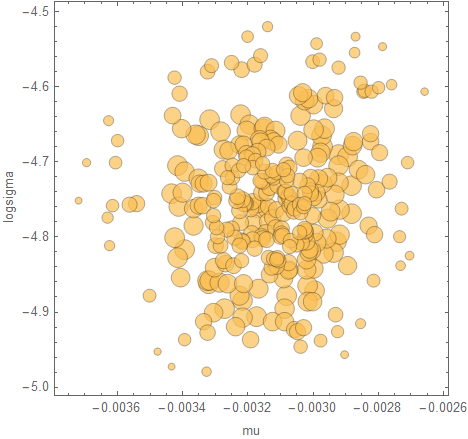
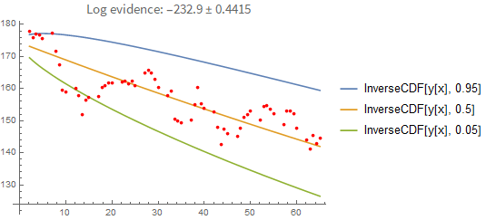
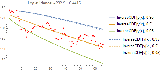
The posterior is mainly useful to have because you can use it to make predictions. Here's a plot of the regression when you "replay" it from the first data point:

predictions = predictiveDistribution[takePosteriorFraction[result, 0.95], ts["Times"]];
plot = regressionPlot1D[result, predictions]

You can also extrapolate from the last known value: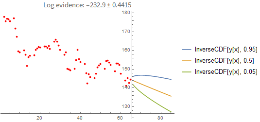

It's instructive to compare these results with a point-estimate using the sample with the highest loglikelihood found. As you can see below, the point-estimate gives a very similar result, so in this case we can conclude that the posterior can be approximated with a single point quite well:

proc = GeometricBrownianMotionProcess[#1, Exp[#2], start] & @@ First[TakeLargestBy[result["Samples"], #LogLikelihood &, 1]]["Point"];
Show[
 plot,
 regressionPlot1D[result, AssociationMap[proc, ts["Times"]], PlotStyle -> Dashed]
 ]

Here is the result if you fit the process properly (i.e., you model each point conditionally on the previous one rather than pretending they are independent of each other). In the first plot you see the prediction error when you predict forward from the last known data point. Again, the dashed line shows you the maximum-likelihood estimate:

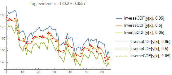
That doesn't seem like a big difference between the two prediction methods. However, this is what happens when you predict forward from the first data point only:

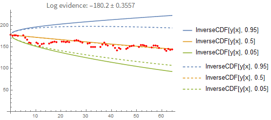
Here the difference between the point-estimate and the full Bayesian prediction becomes more apparent. The point-estimate is too optimistic because it doesn't include the uncertainty in the fitting parameters.

I hope this code is useful to some of you. If you're going to give it a try, please let me know what you think!