I have been for several days now trying to FIndFit some data to a decaying e function:
k[t_] := \[Omega] E^(-((R t)/J))
This function describes a flywheel that starts with an initial velocity and falls to zero. I have a rough estimate of what the friction and the inertia (R and J respectively) of the system should be, but need to verify.
I have several datasets that I'm using to fit with and known initial/boundry conditions, this one for example:
data = {{0.04, 350.73}, {0.44, 342.26}, {0.84, 334.38}, {1.24,
  326.29}, {1.64, 318.2}, {2.04, 310}, {2.44, 302.28}, {2.84,
  294.72}, {3.24, 287.09}, {3.64, 280.08}, {4.04, 272.48}, {4.44,
  265.03}, {4.84, 258.31}, {5.24, 251.15}, {5.64, 244.37}, {6.04,
  237.75}, {6.44, 230.89}, {6.84, 225.03}, {7.24, 218.29}, {7.64,
  212.28}, {8.04, 206.17}, {8.44, 199.7}, {8.84, 193.95}, {9.24,
  188.05}, {9.64, 182.1}, {10.04, 176.14}, {10.44, 170.77}, {10.84,
  165.5}, {11.24, 159.8}, {11.64, 154.4}, {12.04, 148.86}, {12.44,
  143.87}, {12.84, 138.62}, {13.24, 133.58}, {13.64, 128.43}, {14.04,
  123.22}, {14.44, 118.98}, {14.84, 113.85}, {15.24, 109.16}, {15.64,
  104.38}, {16.04, 99.54}, {16.44, 95.2}, {16.84, 90.84}, {17.24,
  86.46}, {17.64, 82}, {18.04, 77.62}, {18.44, 73.43}, {18.84,
  69.11}, {19.24, 65.09}, {19.64, 61.05}, {20.04, 57.17}, {20.44,
  53.06}, {20.84, 48.88}, {21.24, 45.03}, {21.64, 41.29}, {22.04,
  37.4}, {22.44, 33.91}, {22.84, 30.4}, {23.24, 26.59}, {23.64,
  23.02}, {24.04, 19.78}, {24.44, 16}, {24.84, 12.34}, {25.24,
  9.28}, {25.64, 6.17}, {26.04, 4.1}};

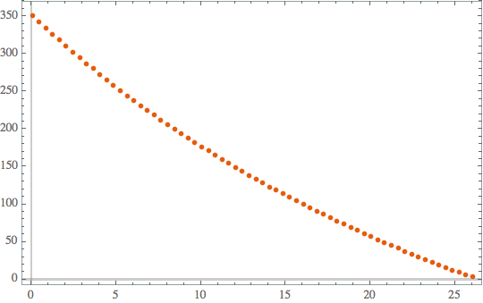
plot2 = ListPlot[data, ImageSize -> Medium, PlotRange -> All,
  PlotTheme -> "Scientific"]

Nothing particularly special.
Whereby omega is equal to 350.73 and the duration of the decay is 26.04 seconds.
I'm trying to find the values for R and J, which should be in a specific range, which you can see in the following FindFit[].
fitparams =
 Join[FindFit[
    data, {k[t] /. \[Omega] -> 350.73, {0.0001 <= R <= 0.0005,
      0.0013 <= J <= 0.0018}}, {R, J}, t] // Flatten, {\[Omega] -> 350.73}]
With a result of:
{R\[Rule]0.00012762656668736746`,J\[Rule]0.0016248495392962767`,\
\[Omega]\[Rule]350.73`}
When trying to plot these to visualize the fit, I get the following plotting error(s):
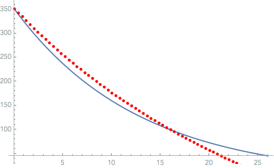
In the image below, the function k[t] approaches zero at 26s like expected, however now the Listplot crosses the x axis just above 20 (and does not terminate at 26.04s like it should) and falls into the negative Y axis...which can't be possible, since there are no negative data points or even ones below 4, for that matter.
Show[Plot[{k[t] /. fitparams}, {t, 0, 26.04}],
 ListPlot[Style[data, Red]], PlotTheme -> "Scientific"]

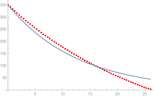
If I switch the order of the plots, now the ListPlot plots correctly, and the function approaches 50 instead of Zero...which is completely wrong.
   Show[ListPlot[Style[data, Red]],
     Plot[{k[t] /. fitparams}, {t, 0, 26.04}],
     PlotTheme -> "Scientific"]

Both the function with calculated R and J and the data display/plot individually how I expect them to, However together with Show[] do not, regardless of order.
Why are the plots not aligning correctly when plotted together, but individually are fine? It's impossible to verify anything.
I greatly appreciate the help!