Message Boards Message Boards

Use FindFit with an exponential function?

Posted 5 years ago

I have been for several days now trying to FIndFit some data to a decaying e function:

k[t_] := \[Omega] E^(-((R t)/J))

This function describes a flywheel that starts with an initial velocity and falls to zero. I have a rough estimate of what the friction and the inertia (R and J respectively) of the system should be, but need to verify.

I have several datasets that I'm using to fit with and known initial/boundry conditions, this one for example:

data = {{0.04, 350.73}, {0.44, 342.26}, {0.84, 334.38}, {1.24, 
  326.29}, {1.64, 318.2}, {2.04, 310}, {2.44, 302.28}, {2.84, 
  294.72}, {3.24, 287.09}, {3.64, 280.08}, {4.04, 272.48}, {4.44, 
  265.03}, {4.84, 258.31}, {5.24, 251.15}, {5.64, 244.37}, {6.04, 
  237.75}, {6.44, 230.89}, {6.84, 225.03}, {7.24, 218.29}, {7.64, 
  212.28}, {8.04, 206.17}, {8.44, 199.7}, {8.84, 193.95}, {9.24, 
  188.05}, {9.64, 182.1}, {10.04, 176.14}, {10.44, 170.77}, {10.84, 
  165.5}, {11.24, 159.8}, {11.64, 154.4}, {12.04, 148.86}, {12.44, 
  143.87}, {12.84, 138.62}, {13.24, 133.58}, {13.64, 128.43}, {14.04, 
  123.22}, {14.44, 118.98}, {14.84, 113.85}, {15.24, 109.16}, {15.64, 
  104.38}, {16.04, 99.54}, {16.44, 95.2}, {16.84, 90.84}, {17.24, 
  86.46}, {17.64, 82}, {18.04, 77.62}, {18.44, 73.43}, {18.84, 
  69.11}, {19.24, 65.09}, {19.64, 61.05}, {20.04, 57.17}, {20.44, 
  53.06}, {20.84, 48.88}, {21.24, 45.03}, {21.64, 41.29}, {22.04, 
  37.4}, {22.44, 33.91}, {22.84, 30.4}, {23.24, 26.59}, {23.64, 
  23.02}, {24.04, 19.78}, {24.44, 16}, {24.84, 12.34}, {25.24, 
  9.28}, {25.64, 6.17}, {26.04, 4.1}};

plot2 = ListPlot[data, ImageSize -> Medium, PlotRange -> All, 
  PlotTheme -> "Scientific"]

correct

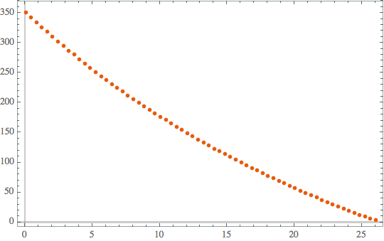
Nothing particularly special.

Whereby omega is equal to 350.73 and the duration of the decay is 26.04 seconds.

I'm trying to find the values for R and J, which should be in a specific range, which you can see in the following FindFit[].

fitparams = 
 Join[FindFit[
    data, {k[t] /. \[Omega] -> 350.73, {0.0001 <= R <= 0.0005, 
      0.0013 <= J <= 0.0018}}, {R, J}, t] // Flatten, {\[Omega] -> 350.73}]

With a result of:

{R\[Rule]0.00012762656668736746`,J\[Rule]0.0016248495392962767`,\
\[Omega]\[Rule]350.73`}

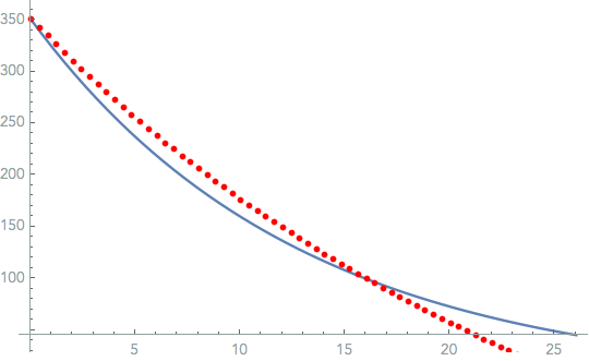
When trying to plot these to visualize the fit, I get the following plotting error(s):

In the image below, the function k[t] approaches zero at 26s like expected, however now the Listplot crosses the x axis just above 20 (and does not terminate at 26.04s like it should) and falls into the negative Y axis...which can't be possible, since there are no negative data points or even ones below 4, for that matter.

Show[Plot[{k[t] /. fitparams}, {t, 0, 26.04}], 
 ListPlot[Style[data, Red]], PlotTheme -> "Scientific"]

weird 1

If I switch the order of the plots, now the ListPlot plots correctly, and the function approaches 50 instead of Zero...which is completely wrong.

   Show[ListPlot[Style[data, Red]], 
     Plot[{k[t] /. fitparams}, {t, 0, 26.04}], 
     PlotTheme -> "Scientific"]

weird 2

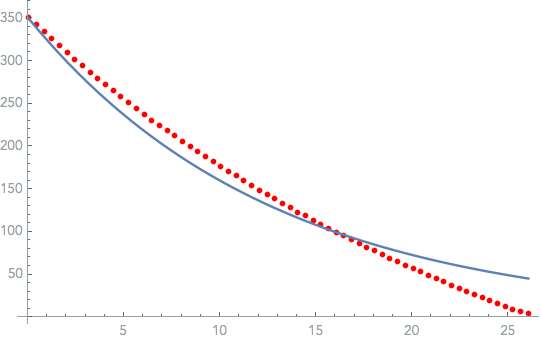
Both the function with calculated R and J and the data display/plot individually how I expect them to, However together with Show[] do not, regardless of order.

Why are the plots not aligning correctly when plotted together, but individually are fine? It's impossible to verify anything.

I greatly appreciate the help!

POSTED BY: Mor Bo
5 Replies

If you plot the data on a log scale, you'll notice that you don't get a straight line:

ListLogPlot[data]

enter image description here

This is a clear indication that a simple decaying exponential is not going to give a good fit to your data.

As a general rule in fitting I highly recommend that, if possible, you always try to plot your data in such a way that your model should give a straight line. If you don't get one, you know immediately that the model is not very good for fitting your data. If you DO get one, fitting is trivial: just fit a straight line to the transformed data and transform back. This will almost always give you a better fit than simply throwing everything into FindFit or NonlinearModelFit. This is especially true for exponential models, which often fit very poorly if you don't log-transform your data even when the data do follow an exponential behaviour.

As an example, consider the following noisy data:

dat = {#, Exp[-(# +  RandomReal[{-1, 1}])]} & /@ Range[0, 20, 0.1];
ListLogPlot[dat]

enter image description here

Fit it two different ways and compare the results:

In[49]:= fit1 = a Exp[k x] /. FindFit[dat, a Exp[k x], {a, k}, x]
fit2 = Exp[Fit[MapAt[Log, dat, {All, 2}], {1, x}, x]]
Show[
 ListLogPlot[dat],
 LogPlot[{fit1, fit2}, {x, 0, 20}]
 ]

Out[49]= 0.711949 E^(-0.659158 x)

Out[50]= E^(0.028229 - 1.00382 x)

enter image description here

As you can see, the fit from FindFit gets thrown off completely. This happens because FindFit minimizes the errors on the linear scale, so it doesn't care about the small values on the right hand side of the plot very much.

POSTED BY: Sjoerd Smit
Posted 5 years ago

Please edit your code. Both time and sdata are undefined. Also, you mention that there are "plotting errors" but show no errors nor is there a description as to what the errors are.

The model and the data can only estimate R/J and not R and J separately. Evidence of this issue (beside observing the structure of the model) is that the estimate of the parameter correlation matrix is singular:

nlm = NonlinearModelFit[data, {k[t] /. \[Omega] -> 350.73, 
  {0.0001 <= R <= 0.0005,  0.0013 <= J <= 0.0018}}, {{R, 0.0003}, {J, 0.0015}}, t]
nlm["BestFitParameters"]
(* {R -> 0.000127627, J -> 0.00162485} *)
nlm["CorrelationMatrix"]
(* {{1., -1.}, {-1., 1.}} *)
POSTED BY: Jim Baldwin
Posted 5 years ago

I have updated the code and described the 'errors' I meant...hopefully my problem is clearer now, Thank you however, for the explanation of the fitting for R/J...I will attempt to find another way to determine the values I need...Do you happen to know why the dataset and the function do not appear to be on the same scale...or atleast why my dataset is plotting in the negative Y, when using Show[] ?

Thanks again for the help!

POSTED BY: Mor Bo
Posted 5 years ago

Ah Thank you for the clear explanation and the examples. I will definitely take it to heart. However, I still have the issue of trying to find approx. values for my R and J...

The original model, for a flywheel driven by electric motor is:

\[Phi][t] -> (t u \[Tau])/R - (E^(-((R t)/J)) J C[1])/R + C[2]

I took the derivative, to get the angular velocity function, as the angle of the flywheel is entirely unknown and not valuable.

Derivative[1][\[Phi]][t] -> (u \[Tau])/R + E^(-((R t)/J)) C[1]

Here, u -> 0 so the first term falls away, C[1] is the initial velocity, R the friction, J the inertia...both values I have a good idea in the range they should be but I need something more accurate...

Do you have a suggestion on how I might find those values? As you say, my data does not give me a straight line when using ListLogPlot...Otherwise I'm at a loss on the best way to find them. Thanks again for the help, I appreciate it!

POSTED BY: Mor Bo
Posted 5 years ago

Hello Mor, your data can be fitted pretty well with the following model:

mod = c[1] Exp[- c[2] (x ) ] + c[3]

Using "NonlinearModelFit" you have to guess good starting parameters for the 3 constants c[i]. From your data plot c[1] =400., c[2] 1./15. and c[3] = 0. is a good 1st guess.

nmf = NonlinearModelFit[data, 
  mod, {Array[c, 3], {400., 1./15., 0.}}\[Transpose], x] 

You can check the fit by plotting against the original data:

ListPlot[Evaluate[{data, {data[[All, 1]], 
     Map[nmf[#] &, data[[All, 1]]]}\[Transpose]}], 
 Joined -> {False, True}, ImageSize -> Large]

enter image description here

POSTED BY: Michael Helmle
Reply to this discussion
Community posts can be styled and formatted using the Markdown syntax.
Reply Preview
Attachments
Remove
or Discard

Group Abstract Group Abstract