curvatureMeasure.m is a Mathematica script for calculating curvature along the boundary of an image object. It might be useful to people working in the computer vision community. This simple script can be easily extended to even track the curvature of an object as it deforms (will add soon) across several images.
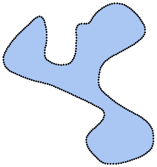
Here is our input image:

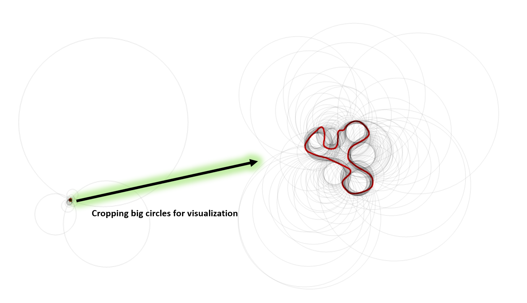
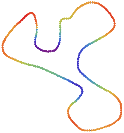
boundary is discretized into equidistant points
circle fits to a given point point Pi, Pi + N-left, Pi + N-right, where N is the neighbour to the point Pi.
curvatures (found as 1/radius) is the colormap:
code
(* ::Package:: *)

BeginPackage["curvatureMeasure`"];


curvatureMeasure::usage = "measures the curvature along the image object";


Begin["`Private`"];


shiftPairs[perimeter_,shift_]:=Module[{newls},
newls=perimeter[[-shift;;]]~Join~perimeter~Join~perimeter[[;;shift]];
Table[{newls[[i-shift]],newls[[i]],newls[[i+shift]]},{i,1+shift,Length[newls]-shift}]
];

(* we can either use the suppressed code below to fit circles or the Built-In Circumsphere to find the fits
(* from Mathematica StackExchange: courtesy ubpdqn *)
circfit[pts_]:=Module[{reg,lm,bf,exp,center,rad},
reg={2 #1,2 #2,#2^2+#1^2}&@@@pts;
lm=LinearModelFit[reg,{1,x,y},{x,y}];
bf=lm["BestFitParameters"];
exp=(x-#2)^2+(y-#3)^2-#1-#2^2-#3^2&@@bf;
{center,rad}={{#2,#3},Sqrt[#2^2+#3^2+#1]}&@@bf;
circlefit[{"expression"->exp,"center"->center,"radius"->rad}]
];
circlefit[list_][field_]:=field/.list;
circlefit[list_]["Properties"]:=list/.Rule[field_,_]:>field;
circlefit/:ReplaceAll[fields_,circlefit[list_]]:=fields/.list;
Format[circlefit[list_],StandardForm]:=HoldForm[circlefit]["<"<>ToString@Length@list<>">"]
*)

curvatureMeasure[img_Image,div_Integer,shift_Integer]:=Module[{\[ScriptCapitalR],polygon,t,interp,sub,sampledPts,
pairedPts,circles,\[Kappa],midpts,regMem,col,g,fn},
\[ScriptCapitalR] = ImageMesh[img, Method -> "Exact"];
polygon = Append[#,#[[1]]]&@MeshCoordinates[\[ScriptCapitalR]][[ MeshCells[\[ScriptCapitalR],2][[1,1]] ]];
t = Prepend[Accumulate[Norm/@Differences[polygon]],0.];
interp = Interpolation[Transpose[{t,polygon}],InterpolationOrder -> 1,
PeriodicInterpolation->True];
sub = Subdivide[interp[[1,1,1]],interp[[1,1,2]],div];
sampledPts = interp[sub];
Print[Show[\[ScriptCapitalR],Graphics@Point@sampledPts,ImageSize-> 250]];
pairedPts = shiftPairs[sampledPts, shift];

circles = (Circumsphere/@pairedPts)/. Sphere -> Circle;
(*circles = (fn=circfit[#]; Circle[fn["center"],fn["radius"]])&/@pairedPts;*)

Print[Graphics[{{Red,Point@sampledPts},{XYZColor[0,0,0,0.1],circles}}]];
\[Kappa] = 1/Cases[circles,x_Circle:> Last@x];
midpts = Midpoint/@pairedPts[[All,{1,-1}]];
regMem = RegionMember[\[ScriptCapitalR],midpts]/.{True-> 1,False-> -1};
\[Kappa] *= regMem;
col = ColorData["Rainbow"]/@Rescale[\[Kappa], MinMax[\[Kappa]],{0,1}];
g = Graphics[{PointSize[0.018],MapThread[Point[#1,VertexColors->#2]&,{sampledPts,col}]}];
Print[Show[HighlightMesh[\[ScriptCapitalR],{Style[1, Black],Style[2,White]}],g,ImageSize->Medium]];
\[Kappa]
]


End[];
EndPackage[];
 Attachments:


