Astroid pedal curves Illustration given in WolframAlpha are parametrized by 3 parameters a, x0 and y0.

If one feeds a simple feedforward network with only the first part of such a curve (e.g. the first 50 points of say 100 points), the natural question arises:

Is it possible to predict the remaining part of the curve with sufficient accuracy?

This can be understood as a sequence-to-sequence prediction.

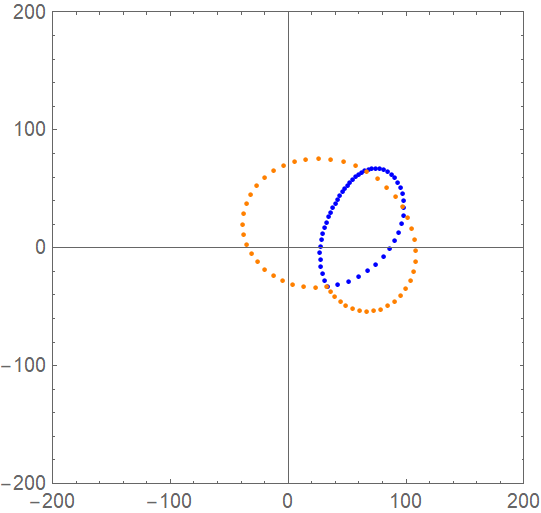
Here is an example how this looks like (orange dots are first part of curve (input data) and blue dots are the second part (output of the net, curve points which should be predicted):

To answer the above question, 100 curves were randomly created for training of the net (training data) and 100 curves as test data. More accurately, the 4 parameters were randomly chosen (see below in source code).

A simple feedforward network based on one linear layer (see details below) was trained and also validated by using 20% as validation set.

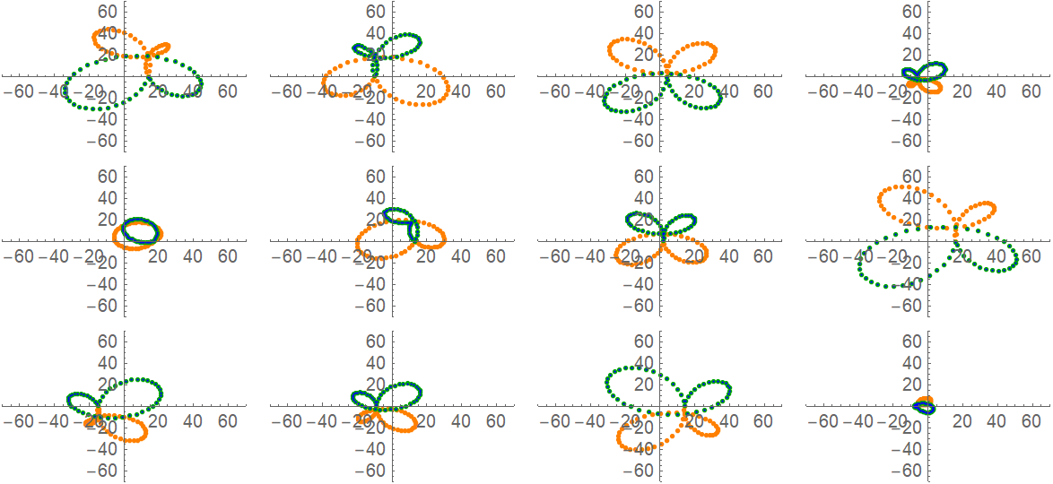
1. The net achieves excellent performance.

Here are some examples: orange (input points), blue (predicted points by the net) and green (points as generated by parameterization of this type of curve)

1. I wonder a bit how it is possible for the net to make such accurate predictions? I think the net "recognizes" that there are only 3 parameters necessary for predictions.

2. I find it remarkable that the net can make such accurate predictions without knowing the underlying parameterization of the curve.

3. here is the source code

   (*Here is the parameterization of the Astroic Pedal Curve*)
   
   AstroidPedalCurve[
     t_, {a_, x0_, y0_}] := {Cos[t] (Sin[t] (a Sin[t] - y0) + x0 Cos[t]),
      Sin[t] (a Cos[2 t] + a - 2 x0 Cos[t] + 2 y0 Sin[t])/2}
   
   (*Illustration of the influence of parameters a, x0 and y0 *)
   
   Manipulate[
    ParametricPlot[AstroidPedalCurve[t, {a, x0, y0}], {t, 0, 2 \[Pi]}, 
     PlotRange -> {{-250, 250}, {-250, 250}}], {a, -200, 200}, {x0, -20, 
     20}, {y0, -20, 20}]
   
   (*Definition of discrete curve points *)
   CurvePoints[{a_, x0_, y0_}] := 
     Table[AstroidPedalCurve[t, {a, x0, y0}], {t, 0, 2 \[Pi], 0.063}];
   
   (*Definition of training and test data for the feedforward net *)
   Clear[data];
   data[k_] := 
     data[k] = 
      TakeDrop[
       CurvePoints[{RandomInteger[{-100, 100}], RandomInteger[{-20, 20}],
          RandomInteger[{-20, 20}]}], 50];
   
   trainingData = <|"input" -> Table[data[k][[1]], {k, 1, 100}], 
      "output" -> Table[data[k][[2]], {k, 1, 100}]|>;
   Clear[independenttestData];
   independenttestData = <|"input" -> Table[data[k][[1]], {k, 201, 300}],
       "output" -> Table[data[k][[2]], {k, 201, 300}]|>;
   
   (*Definition and training of the feedforward net *)
   chain = NetChain[{LinearLayer[{50, 2}, "Output" -> {50, 2}]}]
   model = NetTrain[chain, 
     Thread[trainingData[["input"]] -> trainingData[["output"]]], 
     ValidationSet -> Scaled[0.2]]
   
   (*Illustration of predictions of the net *)
   F[s_, data_] := 
    ListPlot[{data["input"][[s]], data["output"][[s]], 
      model[data["input"][[s]]]}, PlotRange -> {{-70, 70}, {-70, 70}}, 
     PlotStyle -> {{PointSize[0.02], Orange}, {PointSize[0.02], 
        Darker[Green]}, Blue}]
   
   L[k_] := GraphicsGrid[{Table[
       Graphics[F[s, independenttestData]], {s, k, k + 3}],
      Table[Graphics[F[s, independenttestData]], {s, k + 4, k + 7}], 
      Table[Graphics[F[s, independenttestData]], {s, k + 8, k + 11}]}]
   
   L[1]
   

4. BTW, no advanced network layers (e.g. gated recurrent or longshort term layer) are necessary for this type of problem.

5. Have fun playing a bit :-)

6. Finally, I would like to ask the following question:

How is it possible for the net to make so accurate predictions without knowing the underlying parameterization?

Can you explain why? I do not really understand how this works...

with best regards

Wolfgang