I was a teaching assistant for Stewart's Transport class and I took a canoe trip with Bird, but that was 30 years ago so I apologize if the material is not fresh. Mass transport can be tricky, because there are so many species and so many equations to choose form and so many that are not independent. Often, one runs in circles thinking they found a new useful equation only to find it is a combination and re-arrangement of previous equations.
That said, I took a quick look at BSL 2nd edition and I think my original solution is still very close to what you are looking for because:
- It matches initial conditions and boundary conditions well.
- The concentrations profiles tend toward BSL's steady-state solution (eq 18.2-11).
- The solution has Gaussian shaped pulse in molar flux consistent with your error function statement.
- The solution compares favorably to another physics solver.
- Finally, the solution compares favorably to the analytical solution in a short enough time before end effects dominate.
Actually, doing the analysis in the other solver was instructive because it suggested one of the problems with the way you were posing the problem for a numerical solver. Essentially, it reminded me that for each dependent variable, one specifies either Dirichlet (nodal values)
$OR$ Neumann (flux) on the boundary but
$NOT\ BOTH$ (over constraining the system). Since we know the nodal values at the boundaries, the option to specify also a flux went away. This suggests that our method should only contain Dirichlet conditions (the interface concentration
$=x_{sat}$ and the top concentration (equals 0 in this case)) . Other values can be computed as post-processing steps using any of the many relations in BSL that may be constructed from the solution field of NDSolve.
Background
We can rearrange and simplify BSL 18.2-11 (i.e., the steady-state concentration profile) assuming 0 mole fraction at the top to obtain
$${x_A}(z) = 1 - (1 - {{\text{x}}_{A,sat}}){\left( {\frac{1}{{1 - {{\text{x}}_{A,sat}}}}} \right)^\frac{z}{L}}$$
One test of our model would be does it tend toward the correct steady-state profile while matching initial and boundary conditions.
For a semi-infinite system, the analytical solution for concentrations contains error functions. Since molar fluxes are derivatives of concentrations or
$$N_{Az}=\frac{-c{\mathcal{D}_{AB}}}{\left (1-x_A \right )} \frac{\partial x_A}{\partial z} $$ we expect them to be Gaussian like. For a finite domain, we expect it to behave like a Gaussian until the front gets affected by the exit boundary.
Results
I refined my NDSolve to better capture the initial transient effects as shown be the following code:
xsat = Rationalize[ 0.75];
opts = Method -> {"MethodOfLines",
    "SpatialDiscretization" -> {"TensorProductGrid",
      "MinPoints" -> 100, "DifferenceOrder" -> 8}};
eqns = {D[u[t, x], t] + D[-1/(1 - u[t, x])*(D[u[t, x], x]), x] == 0,
   u[0, x] == 0, u[t, 0] == xsat (1 - Exp[-8000 t]), u[t, 1] == 0};
usolh = NDSolveValue[eqns, u, {t, 0, 1}, {x, 0, 1}, opts,
  MaxStepFraction -> 0.0005];
Concentration Profiles
The solution reaches steady-state by about
$t=0.4$ dimensionless time
$t=\frac{t_d \mathcal{D}_{AB}}{L^2}$ units. The following Mathematica code animates the evolution of species concentration to steady-state profiles given by (18.2-11) (Dashed Lines).
legend = SwatchLegend[{Blue, Red}, {"Solvent", "Air"},
   LegendMarkers ->
    Graphics[{EdgeForm[Black], Opacity[0.5], Rectangle[]}],
   LegendLabel -> "Species",
   LegendFunction -> (Framed[#, RoundingRadius -> 5] &),
   LegendMargins -> 5];
ani = Animate[
  Plot[{Callout[1 - usolh[t, x], "B", 0.6,
     CalloutMarker -> "CirclePoint"],
    Callout[usolh[t, x], "A", 0.4, CalloutMarker -> "CirclePoint"],
    xa2[xsat, 1, x], 1 - xa2[xsat, 1, x]}, {x, 0, 1},
   PlotRange -> {0, 1.05},
   PlotStyle -> {Directive[Thick, Red], Directive[Thick, Blue],
     Directive[Dashed, Blue], Directive[Dashed, Red]}, Frame -> True,
   FrameLabel -> {Style["x", 18], Style["u(t,x)", 18],
     Style[StringForm["Concentration Profiles @ t=``", t,
       NumberForm[t, {2, 1}, NumberPadding -> {" ", "0"}]], 18]},
   ImageSize -> Large,
   PlotLegends -> Placed[legend, {Right, Center}]], {t, 0, 0.4,
   0.001}]
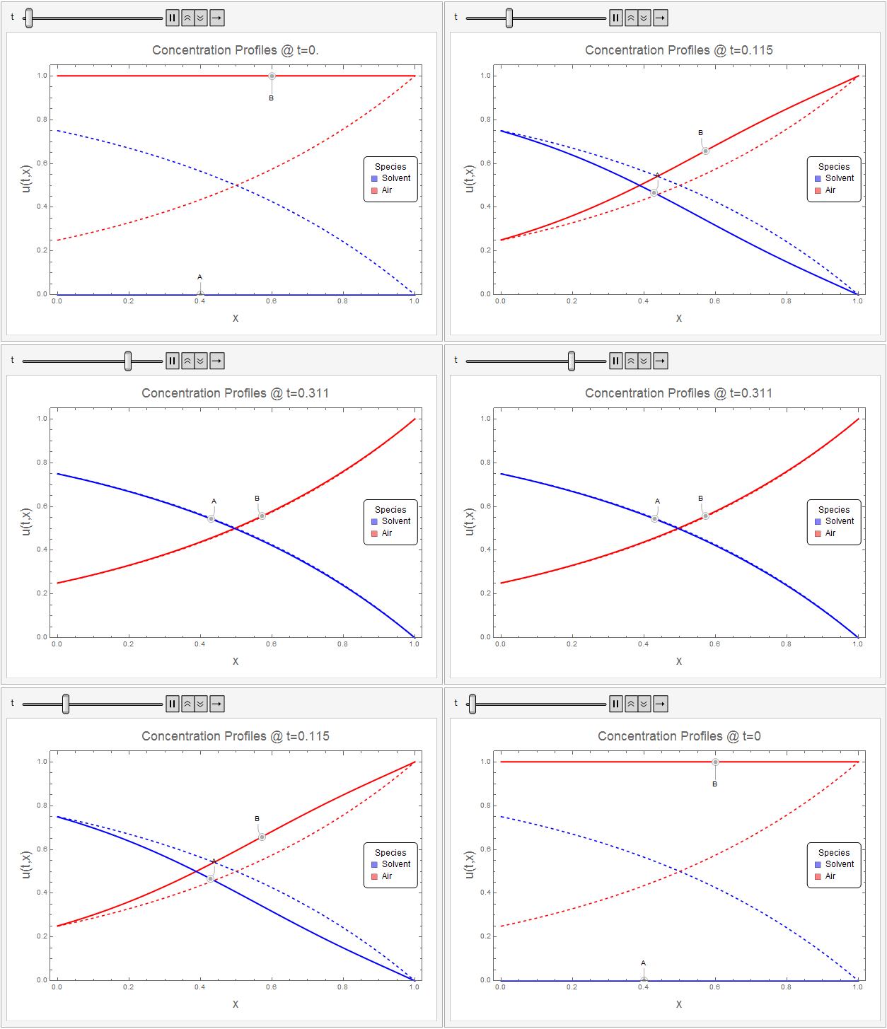
The initial conditions (within the resolution of the concetration ramp) and boundary conditions appear to be well-met. The solution tends towards the steady-state analytical solution quite well.
Flux Profiles
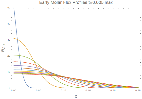
I used the following Mathematica code to view flux evolution at early time. The curves do appear to be Gaussian like at early times before affected by end effects.
Plot[Evaluate[
  Table[(-D[usolh[t, x], x]/(1 - usolh[t, x])) /. {t -> tp,
     x -> xp}, {tp, 0.0001, 0.0055, 0.0005}]], {xp, 0, 0.25},
 PlotRange -> {0, 50}, Frame -> True,
 FrameLabel -> {Style["x", 18], Style["NAz", 18],
   Style[StringForm["Early Molar Flux Profiles t=`` max", 0.005,
     NumberForm[t, {2, 1}, NumberPadding -> {" ", "0"}]], 18]},
 ImageSize -> Large]
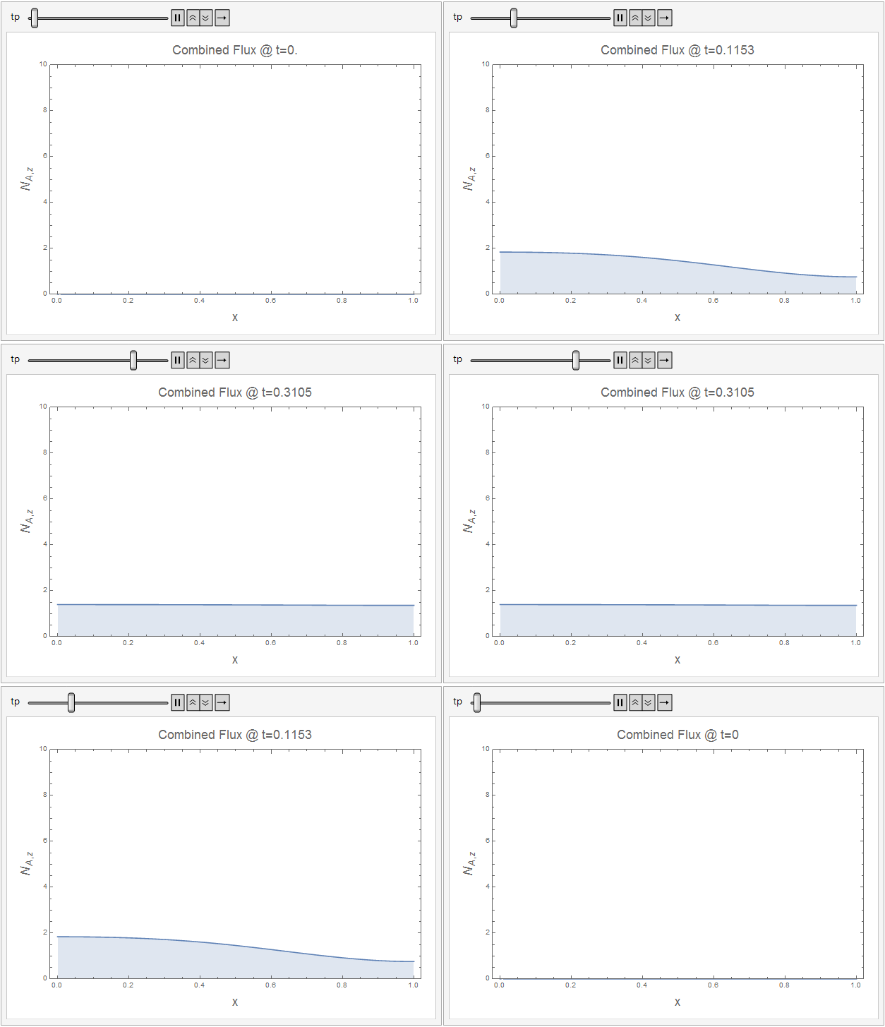
The following code shows how the combined flux approaches a constant value at steady-state.
ani2 = Animate[
  Plot[(-D[usolh[t, x], x]/(1 - usolh[t, x])) /. {t -> tp,
     x -> xp}, {xp, 0, 1}, PlotRange -> {0, 10}, Filling -> Axis,
   Frame -> True,
   FrameLabel -> {Style["x", 18], Style["NAz", 18],
     Style[StringForm["Combined Flux @ t=``", tp,
       NumberForm[t, {2, 1}, NumberPadding -> {" ", "0"}]], 18]},
   ImageSize -> Large], {tp, 0, 0.4, 0.0001}]
Comparison to another Code
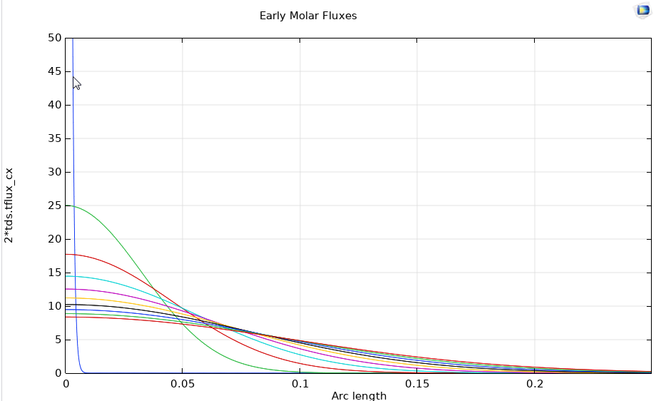
The following compares the Mathematica results to an out-of-the box simulation in COMSOL. This is a quick and dirty test to see qualitatively how the results compare. I did not do a detailed analysis of the equations to make a one-to-one correspondence so the results certainly can vary. The figure below suggests that the results are qualitatively similar.
Comparison to the Semi-Infinite Analytical Solution
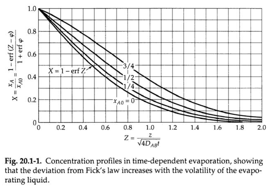
BSL provides a plot of their analytical solution for the semi-infinite case. To facilitate this comparison, we will use ParametricNDSolveValue to parameterize versus
$x_{A0}$.
Clear[xsat]
opts = Method -> {"MethodOfLines",
    "SpatialDiscretization" -> {"TensorProductGrid",
      "MinPoints" -> 100, "DifferenceOrder" -> 8}};
eqns = {D[u[t, x], t] + D[-1/(1 - u[t, x])*(D[u[t, x], x]), x] == 0,
   u[0, x] == 0, u[t, 0] == xsat (1 - Exp[-8000 t]), u[t, 1] == 0};
pfun = ParametricNDSolveValue[eqns, u, {t, 0, 1}, {x, 0, 1}, xsat,
   opts, MaxStepFraction -> 0.0005];
(* Get interpolation functions for plot values *)
usolh75 = pfun[0.75];
usolh50 = pfun[0.5];
usolh25 = pfun[0.25];
Plot[{Callout[usolh75[1/16, 2 Sqrt[1/16] z]/0.75, "3/4", 1,
   CalloutMarker -> "CirclePoint"],
  Callout[usolh50[1/16, 2 Sqrt[1/16] z]/0.5, "1/2", 0.75,
   CalloutMarker -> "CirclePoint"],
  Callout[usolh25[1/16, 2 Sqrt[1/16] z]/0.25, "1/4", 0.5,
   CalloutMarker -> "CirclePoint"]}, {z, 0, 2}, PlotRange -> {0, 1},
 GridLines -> Automatic]
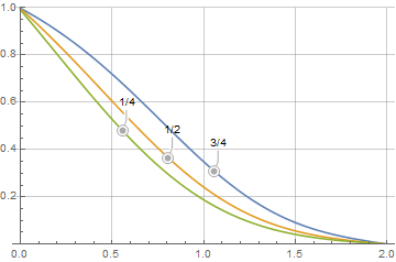
Finally, we compare that with figure 20.1-1 in BSL and we see the results are very similar.
Update
The analytical solution given in BSL, involves some complex inverse functions that, fortunately, Mathematica can calculate quite easily. To create the plot in figure 20.1-1, we need the parameter
$\varphi$, but it is easier to express
$x_{A0}$=
$x_{A0}\left ( \varphi \right )$ as in (20.1-18).
$${x_{A0}} = \frac{1}{{1 + {{\left( {\sqrt \pi \left( {1 + erf\left( \varphi \right)} \right)\varphi \exp \left( {{\varphi ^2}} \right)} \right)}^{ - 1}}}}$$
To obtain
$\varphi$, we need the inverse and an example is given in the FindRoot Documentation and is shown in the Mathematica code below.
inv[f_, s_] := Function[{t}, s /. FindRoot[f - t, {s, 1}]]
xa0[phi_] := 1/(1 + 1/(Sqrt[Pi] (1 + Erf[phi]) phi Exp[phi^2]))
phiinv = inv[xa0[phi], phi]
bigX[Z_, x_] := (1 - Erf[Z - phiinv[x]])/(1 + Erf[phiinv[x]])
Now, we can reproduce Figure 20.1-1 and compare the finite tube to the semi-infinite tube solution using the code below.
frame[legend_] :=
 Framed[legend, FrameStyle -> Red, RoundingRadius -> 10,
  FrameMargins -> 0, Background -> Lighter[LightYellow, 0.25]]
legend = LineLegend[
   Automatic, {"3/4 \[Infinity]", "3/4", "1/2 \[Infinity]", "1/2",
    "1/4 \[Infinity]", "1/4", "0 \[Infinity]"},
   LegendFunction -> frame];
Plot[{bigX[z, 0.75],
  Callout[usolh75[1/16, 2 Sqrt[1/16] z]/0.75, "3/4", 1,
   CalloutMarker -> "CirclePoint"], bigX[z, 0.5],
  Callout[usolh50[1/16, 2 Sqrt[1/16] z]/0.5, "1/2", 0.9,
   CalloutMarker -> "CirclePoint"], bigX[z, 0.25],
  Callout[usolh25[1/16, 2 Sqrt[1/16] z]/0.25, "1/4", 0.8,
   CalloutMarker -> "CirclePoint"], bigX[z, 0]}, {z, 0, 2},
 PlotRange -> {0, 1}, GridLines -> Automatic,
 Filling -> {{1 -> {2}}, {3 -> {4}}, {5 -> {6}}},
 PlotStyle -> {Dashed, Thick, Dashed, Thick, Dashed, Thick, Dashed},
 ImageSize -> Large, Frame -> True,
 FrameLabel -> {Style["Z", 18], Style["X", 18],
   Style[StringForm["Dimensionless Concentration Profiles"], 18]},
 PlotLegends -> Placed[legend, {Right, Center}]]
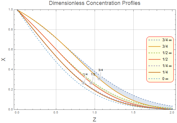
As one can see, the solutions appear similar until they approach the finite boundary and, in that case, the finite tube must approach 0.
Summary
- My initial solution appears to be valid when compared to the semi-infinite solution under appropriate limits.
- I think the problem with the original post was that the system would be over constrained by trying to make the solution obey both Dirichlet and Neumann values on the same boundary.