Message Boards Message Boards

Get numerical solution of PDE for diffusion at high diffusion rates?

I am trying to solve numerically the following PDE with IC and BCs as shown for u(t,x).

\[PartialD]u/\[PartialD]t = \[PartialD]^2u/\[PartialD]x^2 + p Subscript[(\[PartialD]u/\[PartialD]x), x=0]\[PartialD]u/\[PartialD]x
t = 0, u= 0
x= 0, u= 1
x = 1, u = 0

This equation arises in binary diffusion of a species where the diffusion rates are large as opposed to low rates where the second term on the RHS is very small and the PDE becomes identical to the heat conduction equation. This second term accounts for the convective flow induced by the diffusing species. The parameter p is related to the surface concentration of the diffusing species (at x = 0). A closed form solution is available for the case of a semi-infinite region where the last BC becomes x = [Infinity], u = 0. I tried to use NDSolve and NDSolveValue (code shown below) but I got an error message: NDSolveValue::delpde: Delay partial differential equations are not currently supported by NDSolve.

I am unsure if there is (1)a mistake in the code, (2) code is correct but NDSolve cannot provide a solution, or (3) there is a different approach that will work. Would appreciate any help. Thanks.

usolh = NDSolveValue[{D[u[t, x], t] == 
    D[u[t, x], x, x] + 0.5*(D[u[t, x], x] /. x -> 0)*D[u[t, x], x], 
   u[0, x] == 0, u[t, 0] == 1, u[t, 1] == 0}, 
  u, {t, 0, 5}, {x, 0, 1}](*we are assuming p=0.5 here*)
POSTED BY: Rutton Patel
23 Replies

It appears that you are trying to solve the unsteady-state version of the Stefan Tube problem like the figure below where species A is diffusing through stagnant species B.

Stefan Tube

$$\begin{array}{ccccc} N_{A z} & = & -c\mathcal{D}_{A B}\frac{\partial x_A}{\partial z} & + & x_A \left(N_{A z}+N_{B z}\right) \\ \end{array}$$ $$\left\{ {\begin{array}{*{20}{l}} {{\rm{Combined}}}\\ {{\rm{Flux}}} \end{array}} \right\} = \left\{ {\begin{array}{*{20}{l}} {{\rm{Diffusive}}}\\ {{\rm{Flux}}} \end{array}} \right\} + \left\{ {\begin{array}{*{20}{l}} {{\rm{Convective}}}\\ {{\rm{Flux}}} \end{array}} \right\}$$

Since $N_{Bz}$ is zero (stagnant), the equation reduces to

$$N_{A z}=-c\mathcal{D}_{A B}\frac{\partial x_A}{\partial z}+x_A N_{A z}$$

Which can be re-arranged to

$$N_{A z}=-\frac{c \mathcal{D}_{A B}}{1-x_A}\frac{\partial x_A}{\partial z}$$

If in the future you want to use Finite Element Method capabilities, it is conducive to express the equation in coefficient form as shown

$$m\frac{{{\partial ^2}}}{{\partial {t^2}}}u + d\frac{\partial }{{\partial t}}u + \nabla \cdot\left( { - c\nabla u - \alpha u + \gamma } \right) + \beta \cdot\nabla u + au - f = 0$$

The coefficients "c" and "d" are the only non-zero coefficients therefore, we can express your relation as

$$\frac{\partial }{{\partial t}}u + \nabla \cdot\left( { - \frac{1}{1-u}\nabla u } \right) = 0$$

Now, I do not think that you want your parameter $p=0.5$ in the equation, rather that you want to express it as a boundary condition. I added an exponential ramp to eliminate the inconsistent conditions warning.

Re-expressing your relation as Mathematica code, we obtain

usolh = NDSolveValue[{D[u[t, x], t] - 
      D[1/(1 - u[t, x])*(D[u[t, x], x]), x] == 0, u[0, x] == 0, 
    u[t, 0] == 0.5 (1 - Exp[-400 t]), u[t, 1] == 0}, 
   u, {t, 0, 5}, {x, 0, 1}, StartingStepSize -> 0.001];
plt = Plot3D[usolh[t, x], {t, 0., 5.}, {x, 0., 1.}, PlotRange -> All, 
   PlotPoints -> {200, 200}, MaxRecursion -> 4, 
   ColorFunction -> (ColorData["DarkBands"][#3] &), 
   MeshFunctions -> {#2 &}, Mesh -> 20, AxesLabel -> Automatic, 
   MeshStyle -> {Black, Thick}, ImageSize -> Large];
sz = 300;
Grid[{{Show[{plt}, ViewProjection -> "Orthographic", 
    ViewPoint -> Front, ImageSize -> sz, 
    Background -> RGBColor[0.84, 0.92, 1.], Boxed -> False], 
   Show[{plt}, ViewProjection -> "Orthographic", ViewPoint -> Right, 
    ImageSize -> sz, Background -> RGBColor[0.84, 0.92, 1.], 
    Boxed -> False]}, {Show[{plt}, ViewProjection -> "Orthographic", 
    ViewPoint -> Top, ImageSize -> sz, 
    Background -> RGBColor[0.84, 0.92, 1.], Boxed -> False], 
   Show[{plt}, ViewProjection -> "Perspective", 
    ViewPoint -> {Above, Left, Front}, ImageSize -> sz, 
    Background -> RGBColor[0.84, 0.92, 1.], Boxed -> False]}}, 
 Dividers -> Center]

PDE results

After the initial transient, the system achieves steady-state quickly as indicated by the nearly parallel contour lines seen in the lower left image.

POSTED BY: Tim Laska

I was a teaching assistant for Stewart's Transport class and I took a canoe trip with Bird, but that was 30 years ago so I apologize if the material is not fresh. Mass transport can be tricky, because there are so many species and so many equations to choose form and so many that are not independent. Often, one runs in circles thinking they found a new useful equation only to find it is a combination and re-arrangement of previous equations.

That said, I took a quick look at BSL 2nd edition and I think my original solution is still very close to what you are looking for because:

  • It matches initial conditions and boundary conditions well.
  • The concentrations profiles tend toward BSL's steady-state solution (eq 18.2-11).
  • The solution has Gaussian shaped pulse in molar flux consistent with your error function statement.
  • The solution compares favorably to another physics solver.
  • Finally, the solution compares favorably to the analytical solution in a short enough time before end effects dominate.

Actually, doing the analysis in the other solver was instructive because it suggested one of the problems with the way you were posing the problem for a numerical solver. Essentially, it reminded me that for each dependent variable, one specifies either Dirichlet (nodal values) $OR$ Neumann (flux) on the boundary but $NOT\ BOTH$ (over constraining the system). Since we know the nodal values at the boundaries, the option to specify also a flux went away. This suggests that our method should only contain Dirichlet conditions (the interface concentration $=x_{sat}$ and the top concentration (equals 0 in this case)) . Other values can be computed as post-processing steps using any of the many relations in BSL that may be constructed from the solution field of NDSolve.

Background

We can rearrange and simplify BSL 18.2-11 (i.e., the steady-state concentration profile) assuming 0 mole fraction at the top to obtain

$${x_A}(z) = 1 - (1 - {{\text{x}}_{A,sat}}){\left( {\frac{1}{{1 - {{\text{x}}_{A,sat}}}}} \right)^\frac{z}{L}}$$

One test of our model would be does it tend toward the correct steady-state profile while matching initial and boundary conditions.

For a semi-infinite system, the analytical solution for concentrations contains error functions. Since molar fluxes are derivatives of concentrations or $$N_{Az}=\frac{-c{\mathcal{D}_{AB}}}{\left (1-x_A \right )} \frac{\partial x_A}{\partial z} $$ we expect them to be Gaussian like. For a finite domain, we expect it to behave like a Gaussian until the front gets affected by the exit boundary.

Results

I refined my NDSolve to better capture the initial transient effects as shown be the following code:

xsat = Rationalize[ 0.75];
opts = Method -> {"MethodOfLines", 
    "SpatialDiscretization" -> {"TensorProductGrid", 
      "MinPoints" -> 100, "DifferenceOrder" -> 8}};
eqns = {D[u[t, x], t] + D[-1/(1 - u[t, x])*(D[u[t, x], x]), x] == 0, 
   u[0, x] == 0, u[t, 0] == xsat (1 - Exp[-8000 t]), u[t, 1] == 0};
usolh = NDSolveValue[eqns, u, {t, 0, 1}, {x, 0, 1}, opts, 
  MaxStepFraction -> 0.0005];

Concentration Profiles

The solution reaches steady-state by about $t=0.4$ dimensionless time $t=\frac{t_d \mathcal{D}_{AB}}{L^2}$ units. The following Mathematica code animates the evolution of species concentration to steady-state profiles given by (18.2-11) (Dashed Lines).

legend = SwatchLegend[{Blue, Red}, {"Solvent", "Air"}, 
   LegendMarkers -> 
    Graphics[{EdgeForm[Black], Opacity[0.5], Rectangle[]}], 
   LegendLabel -> "Species", 
   LegendFunction -> (Framed[#, RoundingRadius -> 5] &), 
   LegendMargins -> 5];
ani = Animate[
  Plot[{Callout[1 - usolh[t, x], "B", 0.6, 
     CalloutMarker -> "CirclePoint"], 
    Callout[usolh[t, x], "A", 0.4, CalloutMarker -> "CirclePoint"], 
    xa2[xsat, 1, x], 1 - xa2[xsat, 1, x]}, {x, 0, 1}, 
   PlotRange -> {0, 1.05}, 
   PlotStyle -> {Directive[Thick, Red], Directive[Thick, Blue], 
     Directive[Dashed, Blue], Directive[Dashed, Red]}, Frame -> True, 
   FrameLabel -> {Style["x", 18], Style["u(t,x)", 18], 
     Style[StringForm["Concentration Profiles @ t=``", t, 
       NumberForm[t, {2, 1}, NumberPadding -> {" ", "0"}]], 18]}, 
   ImageSize -> Large, 
   PlotLegends -> Placed[legend, {Right, Center}]], {t, 0, 0.4, 
   0.001}]

Concentration Profiles

The initial conditions (within the resolution of the concetration ramp) and boundary conditions appear to be well-met. The solution tends towards the steady-state analytical solution quite well.
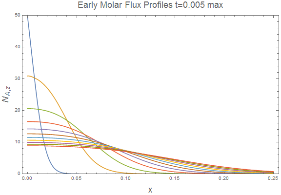
Flux Profiles

I used the following Mathematica code to view flux evolution at early time. The curves do appear to be Gaussian like at early times before affected by end effects.

Plot[Evaluate[
  Table[(-D[usolh[t, x], x]/(1 - usolh[t, x])) /. {t -> tp, 
     x -> xp}, {tp, 0.0001, 0.0055, 0.0005}]], {xp, 0, 0.25}, 
 PlotRange -> {0, 50}, Frame -> True, 
 FrameLabel -> {Style["x", 18], Style["NAz", 18], 
   Style[StringForm["Early Molar Flux Profiles t=`` max", 0.005, 
     NumberForm[t, {2, 1}, NumberPadding -> {" ", "0"}]], 18]}, 
 ImageSize -> Large]

Mathematica Flux Profiles

The following code shows how the combined flux approaches a constant value at steady-state.

ani2 = Animate[
  Plot[(-D[usolh[t, x], x]/(1 - usolh[t, x])) /. {t -> tp, 
     x -> xp}, {xp, 0, 1}, PlotRange -> {0, 10}, Filling -> Axis, 
   Frame -> True, 
   FrameLabel -> {Style["x", 18], Style["NAz", 18], 
     Style[StringForm["Combined Flux @ t=``", tp, 
       NumberForm[t, {2, 1}, NumberPadding -> {" ", "0"}]], 18]}, 
   ImageSize -> Large], {tp, 0, 0.4, 0.0001}]

Steady Flux Evolution

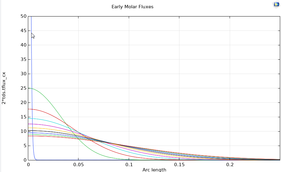
Comparison to another Code

The following compares the Mathematica results to an out-of-the box simulation in COMSOL. This is a quick and dirty test to see qualitatively how the results compare. I did not do a detailed analysis of the equations to make a one-to-one correspondence so the results certainly can vary. The figure below suggests that the results are qualitatively similar.

enter image description here

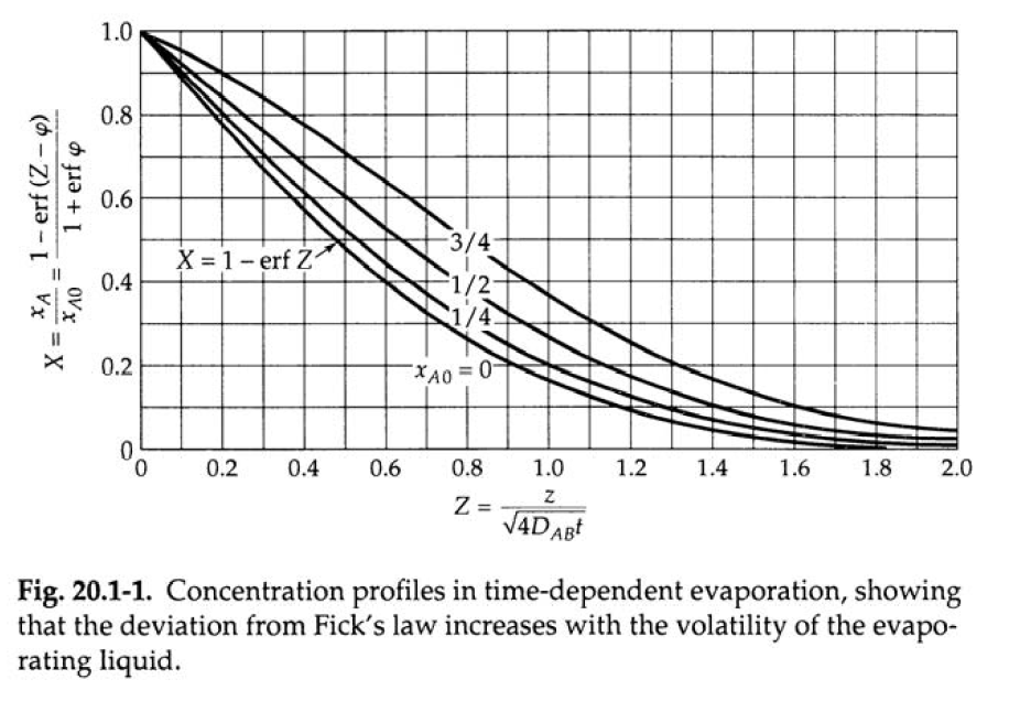
Comparison to the Semi-Infinite Analytical Solution

BSL provides a plot of their analytical solution for the semi-infinite case. To facilitate this comparison, we will use ParametricNDSolveValue to parameterize versus $x_{A0}$.

Clear[xsat]
opts = Method -> {"MethodOfLines", 
    "SpatialDiscretization" -> {"TensorProductGrid", 
      "MinPoints" -> 100, "DifferenceOrder" -> 8}};
eqns = {D[u[t, x], t] + D[-1/(1 - u[t, x])*(D[u[t, x], x]), x] == 0, 
   u[0, x] == 0, u[t, 0] == xsat (1 - Exp[-8000 t]), u[t, 1] == 0};
pfun = ParametricNDSolveValue[eqns, u, {t, 0, 1}, {x, 0, 1}, xsat, 
   opts, MaxStepFraction -> 0.0005];
(* Get interpolation functions for plot values *)
usolh75 = pfun[0.75];
usolh50 = pfun[0.5];
usolh25 = pfun[0.25];
Plot[{Callout[usolh75[1/16, 2 Sqrt[1/16] z]/0.75, "3/4", 1, 
   CalloutMarker -> "CirclePoint"], 
  Callout[usolh50[1/16, 2 Sqrt[1/16] z]/0.5, "1/2", 0.75, 
   CalloutMarker -> "CirclePoint"], 
  Callout[usolh25[1/16, 2 Sqrt[1/16] z]/0.25, "1/4", 0.5, 
   CalloutMarker -> "CirclePoint"]}, {z, 0, 2}, PlotRange -> {0, 1}, 
 GridLines -> Automatic]

Figure 20.1-1 Simulated

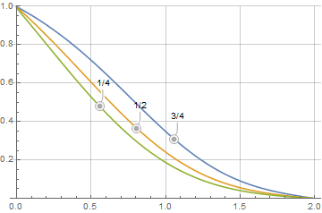
Finally, we compare that with figure 20.1-1 in BSL and we see the results are very similar.

BSL Figure 20.1-1

Update

The analytical solution given in BSL, involves some complex inverse functions that, fortunately, Mathematica can calculate quite easily. To create the plot in figure 20.1-1, we need the parameter $\varphi$, but it is easier to express $x_{A0}$= $x_{A0}\left ( \varphi \right )$ as in (20.1-18).

$${x_{A0}} = \frac{1}{{1 + {{\left( {\sqrt \pi \left( {1 + erf\left( \varphi \right)} \right)\varphi \exp \left( {{\varphi ^2}} \right)} \right)}^{ - 1}}}}$$

To obtain $\varphi$, we need the inverse and an example is given in the FindRoot Documentation and is shown in the Mathematica code below.

inv[f_, s_] := Function[{t}, s /. FindRoot[f - t, {s, 1}]]
xa0[phi_] := 1/(1 + 1/(Sqrt[Pi] (1 + Erf[phi]) phi Exp[phi^2]))
phiinv = inv[xa0[phi], phi]
bigX[Z_, x_] := (1 - Erf[Z - phiinv[x]])/(1 + Erf[phiinv[x]])

Now, we can reproduce Figure 20.1-1 and compare the finite tube to the semi-infinite tube solution using the code below.

frame[legend_] := 
 Framed[legend, FrameStyle -> Red, RoundingRadius -> 10, 
  FrameMargins -> 0, Background -> Lighter[LightYellow, 0.25]]
legend = LineLegend[
   Automatic, {"3/4 \[Infinity]", "3/4", "1/2 \[Infinity]", "1/2", 
    "1/4 \[Infinity]", "1/4", "0 \[Infinity]"}, 
   LegendFunction -> frame];
Plot[{bigX[z, 0.75], 
  Callout[usolh75[1/16, 2 Sqrt[1/16] z]/0.75, "3/4", 1, 
   CalloutMarker -> "CirclePoint"], bigX[z, 0.5], 
  Callout[usolh50[1/16, 2 Sqrt[1/16] z]/0.5, "1/2", 0.9, 
   CalloutMarker -> "CirclePoint"], bigX[z, 0.25], 
  Callout[usolh25[1/16, 2 Sqrt[1/16] z]/0.25, "1/4", 0.8, 
   CalloutMarker -> "CirclePoint"], bigX[z, 0]}, {z, 0, 2}, 
 PlotRange -> {0, 1}, GridLines -> Automatic, 
 Filling -> {{1 -> {2}}, {3 -> {4}}, {5 -> {6}}}, 
 PlotStyle -> {Dashed, Thick, Dashed, Thick, Dashed, Thick, Dashed}, 
 ImageSize -> Large, Frame -> True, 
 FrameLabel -> {Style["Z", 18], Style["X", 18], 
   Style[StringForm["Dimensionless Concentration Profiles"], 18]}, 
 PlotLegends -> Placed[legend, {Right, Center}]]

Direct comparison of finite versus semi-infinite

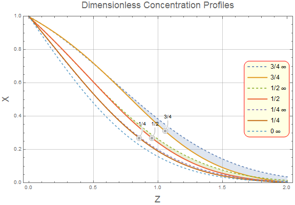
As one can see, the solutions appear similar until they approach the finite boundary and, in that case, the finite tube must approach 0.

Summary

  • My initial solution appears to be valid when compared to the semi-infinite solution under appropriate limits.
  • I think the problem with the original post was that the system would be over constrained by trying to make the solution obey both Dirichlet and Neumann values on the same boundary.
POSTED BY: Tim Laska

I will add the following for completeness. If you read the The Numerical Method of Lines Tutorial, it shows you how you can roll your own discretization scheme using NDSolve`FiniteDifferenceDerivative to accomplish what you need.

Use equations 19.1-12 and 19.1-13 from BSL to reduce $\mathbf{v}^*=f(t\ only)$ as shown:

$$\frac{{\partial c}}{{\partial t}} = - \left( {\nabla \cdot c{\mathbf{v}^*}} \right) + \sum\limits_{\alpha = 1}^N {{R_\alpha }} \qquad (19.1-12) $$

$$ \left( {\nabla \cdot {\mathbf{v}^*}} \right) =\frac{1}{c} \sum\limits_{\alpha = 1}^N {{R_\alpha }} \qquad (19.1-13) $$

$$\left( {\nabla \cdot {{\mathbf{v}}^*}} \right) = 0$$

Since the divergence of $\mathbf{v}^*$ is zero and this is a 1-d problem it means this value is a constant with respect to $z$. Equation (19.1-17) simplifies to the boxed form for a non-reactive system.

$$c\left( {\frac{{\partial {x_\alpha }}}{{\partial t}} + \left( {{{\mathbf{v}}^*} \cdot \nabla {x_\alpha }} \right)} \right) = c{\mathcal{D}_{AB}}{\nabla ^2}{x_A} + \left( {{x_B}{R_A} - {x_A}{R_B}} \right) \qquad (19.1-17) $$

$$\boxed{\left( {\frac{{\partial {x_\alpha }}}{{\partial t}} + \left( {{{\mathbf{v}}^*} \cdot \nabla {x_\alpha }} \right)} \right) = {\mathcal{D}_{AB}}{\nabla ^2}{x_A}}$$

Now, we need to solve for $\mathbf{v}^*$, which is defined by

$$\mathbf{v}^*=\frac{N_A+N_B}{c}$$

Since $\frac{N_A+N_B}{c}$ does not depend on $z$, we choose the interface condition where $N_B$ equals 0 similar to the situation of steady-state and we obtain the same relation for $N_A$.

$$N_{A z}=-\frac{c \mathcal{D}_{A B}}{1-x_A}\frac{\partial x_A}{\partial z}$$

By rolling our own scheme, we have access to the derivative at the boundary. The following shows the Mathematica implementation and evaluation of the boxed equation evaluated up to $\frac{1}{4}$ length.

molMod[x_, ramp_, tmax_] := 
 Module[{n, h , sf, U, bc0, bc0d , bc1, bc1d, delconc, laplacianconc, 
   vstar, eqns, ics, system, lines, f, xsat, m},
  n = 50; Subscript[h, n] = 1/n; sf = 1;
  xsat = Rationalize[x];
  m = Rationalize[ramp];
  U[t_] = Table[Subscript[u, i][t], {i, 0, n}];
  bc0 = Subscript[u, 0][t] == xsat (1 - Exp[-m t]);
  bc0d = Map[D[#, t] + sf # &, bc0];
  bc1 = Subscript[u, n][t] == 0;
  bc1d = Map[D[#, t] + sf # &, bc1];
  delconc = 
   NDSolve`FiniteDifferenceDerivative[1, Subscript[h, n] Range[0, n], 
    U[t]];
  laplacianconc = 
   NDSolve`FiniteDifferenceDerivative[2, Subscript[h, n] Range[0, n], 
    U[t]];
  vstar = -1/(1 - Subscript[u, 0][t]) delconc[[1]];
  eqns = Thread[D[U[t], t] + vstar delconc -  laplacianconc == 0];
  eqns[[1]] = bc0d;
  eqns[[-1]] = bc1d;
  ics = Thread[U[0] == Table[0, {n + 1}]];
  system = Join[eqns, ics];
  lines = NDSolve[system, U[t], {t, 0, 1}];
  f = Interpolation[
    Flatten[Table[{{t, i Subscript[h, n]}, 
       First[Subscript[u, i][t] /. lines]}, {i, 0, n}, {t, 0, tmax, 
       tmax/500}], 1], InterpolationOrder -> 2];
  f]
f75 = molMod[0.75, 20000, 0.01];
f50 = molMod[0.5, 20000, 0.01];
f25 = molMod[0.25, 20000, 0.01];
inv[f_, s_] := Function[{t}, s /. FindRoot[f - t, {s, 1}]]
xa0[phi_] := 1/(1 + 1/(Sqrt[Pi] (1 + Erf[phi]) phi Exp[phi^2]))
phiinv = inv[xa0[phi], phi];
bigX[Z_, x_] := (1 - Erf[Z - phiinv[x]])/(1 + Erf[phiinv[x]])
frame[legend_] := 
 Framed[legend, FrameStyle -> Red, RoundingRadius -> 10, 
  FrameMargins -> 0, Background -> Lighter[LightYellow, 0.25]]
legend = LineLegend[
   Automatic, {"3/4 \[Infinity]", "3/4", "1/2 \[Infinity]", "1/2", 
    "1/4 \[Infinity]", "1/4", "0 \[Infinity]"}, 
   LegendFunction -> frame];
Plot[{bigX[z, 0.75], 
  Callout[f75[1/256, 2 Sqrt[1/256] z]/0.75, "3/4", 1, 
   CalloutMarker -> "CirclePoint"], bigX[z, 0.5], 
  Callout[f50[1/256, 2 Sqrt[1/256] z]/0.5, "1/2", 0.9, 
   CalloutMarker -> "CirclePoint"], bigX[z, 0.25], 
  Callout[f25[1/256, 2 Sqrt[1/256] z]/0.25, "1/4", 0.8, 
   CalloutMarker -> "CirclePoint"], bigX[z, 0]}, {z, 0, 2}, 
 PlotRange -> {0, 1}, GridLines -> Automatic, 
 Filling -> {{1 -> {2}}, {3 -> {4}}, {5 -> {6}}}, 
 PlotStyle -> {Dashed, Thick, Dashed, Thick, Dashed, Thick, Dashed}, 
 ImageSize -> Large, Frame -> True, 
 FrameLabel -> {Style["Z", 18], Style["X", 18], 
   Style[StringForm["Dimensionless Concentration Profiles"], 18]}, 
 PlotLegends -> Placed[legend, {Right, Center}]]

Custom Method of Lines Solution

Very tight agreement with the semi-infinite case. The following plot shows how different the new custom formulation (dashed lines) is versus my initial quick and dirty model (solid lines).

Method comparison

There looks to be about a 10% error that exists at dimensionless time scales between 0.05-0.15. In the end, one needs to operate within the constraints of the currently available solver. Mathematica 11.3 has the capability to solve this case, but you probably will need to do a deep dive into the MOL tutorial and start with a different form of the balance equation.

POSTED BY: Tim Laska

enter image description here

POSTED BY: Rutton Patel
Posted 5 years ago

I have both editions, but it has been a couple or more decades since I have read those sections. I will revisit it when I have a few moments.

Personally, I have not seen cases where there is something that looks like a boundary condition expressed in the main equation in NDSolve. That was some cleverness that BSL applied in the 60s before the advent of Computer Algebra Systems and probably is not appropriate for a general purpose PDE solver like NDSolve.

You may be able to express your problem as a system of PDEs $x_A, N_A, N_B$ since you know initial and boundary concentrations and you know that $N_B$ equals zero at $z=0$.

I will take another look when I have a spare moment if nobody else chimes in.

POSTED BY: Updating Name

The solution given in BSL dates to 1944! For the semi-infinite domain in z the exact solution is in terms of error functions. Thanks again!

POSTED BY: Rutton Patel

enter image description here

POSTED BY: Rutton Patel

Hi Rutton,

I would say that the answer to your question (1) is probably yes there is a mistake in your formulation at least at this time because your derivative term evaluated at the boundary is infinite at $t=0$. The condition that you imposed would look like UnitStep[-x] at $t=0$.

unit step

Mathematica says this is indeterminate.

(D[UnitStep[-x], x] /. x -> 0) (*  Indeterminate *)

When you execute your code, you get the warning

NDSolveValue::delpde: Delay partial differential equations are not currently supported by NDSolve.

Perhaps, that is what you need to get beyond your infinite term at $t=0$, but it is not implement yet. What is interesting, is that since the derivative at the boundary is proportional to molar velocity, and it would be physically impossible to have infinite velocity.

Best regards,

Tim

POSTED BY: Tim Laska

Dear Tim,

Your point is well taken and I will think more about it. The MMA tutorial on DDE does not cover PDEs and the examples for ODEs do not contain terms involving the gradient at 0. I guess it is a question to pose to MMA developers.

Thanks, best regards and HAPPY NEW YEAR!

Rutton

POSTED BY: Rutton Patel

Rutton,

At this year's Wolfram Conference, Wolfram developer, Yi-Lin Chiu demonstrated how to handle PDE's for acoustics. While your PDE's will be a bit different, I think this talk will be helpful for generally solving PDE's relating space and time with various boundary conditions in Mathematica.

On this page- search for Modeling Acoustics with Differential Equations

You can use his notebook as a tutorial. I did not compare it to your example, I'd be curious if you find it helpful.

Regards,

Neil

POSTED BY: Neil Singer

@Rutton D Patel, welcome to Wolfram Community! Please make sure you know the rules:

https://wolfr.am/READ-1ST

The rules explain how to format your posts properly. We believe if you read this short guide you will have no problems with posting, as all other members of Community have no trouble with it. We do not except text and code as images in most of the cases. Please in future follow the rules for the proper formatting of your posts.

POSTED BY: Moderation Team

Neil,

Thanks very much for your suggestion. I have been away, hence the delayed response. I will look at Yi-Lin Chiu's NB.

Regards,

Rutton

POSTED BY: Rutton Patel
Posted 5 years ago

I am still puzzled that the solution to your equation should match so closely with the semi-infinite case for a different equation - the one in BSL. The problem that I have with your equation as I stated previously is that while $N_B$ is 0 at the interface, it is NOT $0$ everywhere during the transient. Therefore the rate relation $$N_{A z}=-\frac{c \mathcal{D}_{A B}}{1-x_A}\frac{\partial x_A}{\partial z}$$ is incorrect everywhere except at the interface. As a consequence I think that your PDE will not satisfy mass conservation during the transient. I also come to this conclusion from a physical argument as follows.

At time < 0, the space above the interface has $x_A$ = 0 and $x_B$ = 1 everywhere. At time 0+ evaporation of $A$ begins at the interface so we have a flux of $A$ along the tube. To satisfy mass conservation, some $B$ must leave and $N_B$ must be non-zero along the tube length.

I tried to find why the two solutions appear to match by examining your code (never easy to do for someone else's code!) and have a question about the horizontal axis on your figure labeled "Dimensionless Concentration Profiles". For the BSL solution curves (I like the neat way you used the Mathematica "inv" to solve for phi as a function of $x_{\text{A0}}$) the horizontal axis variable is the dimensionless variable $Z$ defined as $\frac{z}{2 \sqrt{t D_{\text{AB}}}}$ where $z$ is the dimensional distance, $t$ is dimensional time and $D_{\text{AB}}$ is the diffusivity. Can you clarify what the horizontal axis is for the curves from your solution and where this is coded?

Thanks again for your help and interest.

POSTED BY: Updating Name

By rolling your own Method Of Lines (MOL), you get more flexibility on what you can do with the derivatives. If you look at "vstar", then you see it was only evaluated at the interface $u_0$ (note that part 1 of delconc is also at the interface).

vstar = -1/(1 - Subscript[u, 0][t]) delconc[[1]];

So, vstar is evaluated at the interface only where the flux of B is zero and it is only a function of $t$ because its divergence is zero. Therefore, it should satisfy your conditions of only being evaluated at the interface and not throughout the domain.

Regarding the figure 20.1-1, if the characteristic length scale is, $L$, and the characteristic time scale is $\frac{L^2}{D_{AB}}$, then Z using dimensionless units becomes

$$Z=\frac{z}{\sqrt{4t}}$$

Given that figure 20.1-1 has a Z value that goes from 0 to 2 and we know that z is between 0 and 1, we can solve for t in terms of z.

Solve[z/(2*Sqrt[t]) == 2, t]
(* {{t -> z^2/16}} *)

So, I chose $z=\frac{1}{4}<1$ and that meant the time when $Z=2$ was $t=\frac{1}{256}$. Then, I solved for $z$ in terms of $Z$ using.

Solve[bigZ == z/(2*Sqrt[t]), z]
(* {{z -> 2*bigZ*Sqrt[t]}} *)

Taken together, that means the following is the numerically derived $X$ for $x_{A0}=0.5$ @ $z=\frac{1}{4}$ (note that z in the Mathematica implementation is actually $Z$ to avoid beginning with capitals).

f50[1/256, 2 Sqrt[1/256] z]/0.5

If we want to look at the case where $z=1$, then $t=\frac{1}{16}$. Now, instead of following the infinite tube, we expect the numerical result to satisfy the $x_{A0}=0$ boundary condition.

Plot[{bigX[z, 0.75], 
  Callout[f75[1/16, 2 Sqrt[1/16] z]/0.75, "3/4", 1, 
   CalloutMarker -> "CirclePoint"], bigX[z, 0.5], 
  Callout[f50[1/16, 2 Sqrt[1/16] z]/0.5, "1/2", 0.9, 
   CalloutMarker -> "CirclePoint"], bigX[z, 0.25], 
  Callout[f25[1/16, 2 Sqrt[1/16] z]/0.25, "1/4", 0.8, 
   CalloutMarker -> "CirclePoint"], bigX[z, 0]}, {z, 0, 2}, 
 PlotRange -> {0, 1}, GridLines -> Automatic, 
 Filling -> {{1 -> {2}}, {3 -> {4}}, {5 -> {6}}}, 
 PlotStyle -> {Dashed, Thick, Dashed, Thick, Dashed, Thick, Dashed}, 
 ImageSize -> Large, Frame -> True, 
 FrameLabel -> {Style["Z", 18], Style["X", 18], 
   Style[StringForm["Dimensionless Concentration Profiles"], 18]}, 
 PlotLegends -> Placed[legend, {Right, Center}]]

z equal 1 case

It appears that the BC is satisfied.

Now, we can test your assertion that my model does not allow for mass conservation by simply evaluating $N_{Bz}$ at $z=1$. You can use the relations stated previously to derive an expression for the molar flux of B. Start with the dimensionless molar velocity.

$$\mathbf{v}^*=N_A+N_B$$

Use the expression for $N_{B z}$ in terms of $x_A$. $$N_{B z} = \left (1-x_A \right ) \left(N_{A z}+N_{B z}\right)+\frac{\partial x_A}{\partial z} $$

Substitute $\mathbf{v}^*$ for $N_A+N_B$ $$N_{B z} = \left (1-x_A \right ) \mathbf{v}^*+\frac{\partial x_A}{\partial z}$$

Evaluate at the exit ( $z=1$).

$${N_{Bz}} = {\left. {\left( {1 - {x_A}} \right){{\mathbf{v}}^*} + \frac{{\partial {x_A}}}{{\partial z}}} \right|_{z = 1}}$$

Evaluate $\mathbf{v}^*$ at the interface $${N_{Bz}} = {\left. {\left( {\left( {1 - {x_A}} \right)\left( {{{\left. {\frac{1}{{1 - {x_{A,sat}}}}\frac{{\partial {x_A}}}{{\partial z}}} \right|}_{z = 0}}} \right) + \frac{{\partial {x_A}}}{{\partial z}}} \right)} \right|_{z = 1}}$$

We can implement and plot the last equation in Mathematica code for the $x_{A,sat}=0.5$ case.

Plot[((1 - f50[t, 1]) (-D[f50[t, x], x]/(1 - 0.5)) /. {t -> tp, 
     x -> 0}) + ((D[f50[t, x], x]) /. {t -> tp, x -> 1}), {tp, 0.0002,
   0.1}, PlotRange -> {-1, 40}, ImageSize -> Large, Frame -> True, 
 FrameLabel -> {Style["Dimensionless Time", 18], 
   Style["\!\(\*SubscriptBox[\(N\), \(Bz\)]\)", 18], 
   Style[StringForm["Flux of B at z=1"], 18]}]

enter image description here

Now, we did not achieve infinite flux because this is a numerical model, but the flux of B at the exit starts out very high and asymptotically approaches 0 at large t. So, the assertion of the model having zero B flux along the axis is false.

POSTED BY: Tim Laska

Thanks very much for the clarification of your code and method. If as you say "vstar" is evaluated only at the interface my objection is inapplicable. I misunderstood in thinking that you were still solving the PDE in your first post which is valid only when $B$ is stagnant for all $z$. I find your code very ingeneous particularly in comparing your results with the semi-infinite case!

In comparing your solution to the semi-infinite solution from BSL, I wonder if you compared your values of vstar to the BSL $\phi$ (which is the same as vstar) for various $x_{\text{A0}}$? That would be very interesting.

Thanks again for your help and interest in this problem.

POSTED BY: Rutton Patel

Thank you Rutton!

Since $Z$ is a combined variable of z and t, I think you need to multiply the $\phi$ expression by $\sqrt{t}$ to make it equivalent to dimensionless $\mathbf{v}^*$. If we choose the $t=\frac{1}{256}$ again, then we can plot the numerically derived result versus the analytical solution using:

Plot[phiinv[x], {x, 0.01, 0.99}, ImageSize -> Large, Frame -> True, 
 FrameLabel -> {Style["xa0", 18], Style["\[Phi]", 18], 
   Style[StringForm["Dimensionless Interface Flux"], 18]}, 
 Epilog -> {PointSize[0.02], 
   Point[{0.25, ((-Sqrt[t] D[f25[t, x], x])/(1 - 0.25))}] /. {t -> 
      1/256, x -> 0}, 
   Point[{0.5, ((-Sqrt[t] D[f50[t, x], x])/(1 - 0.5))}] /. {t -> 
      1/256, x -> 0}, 
   Point[{0.75, ((-Sqrt[t] D[f75[t, x], x])/(1 - 0.75))}] /. {t -> 
      1/256, x -> 0}}]

Phi comparison

You can see very tight agreement between the analytical our numerical solution for the evaluated points.

POSTED BY: Tim Laska
Posted 5 years ago

Very encouraging results, Tim. Really neat and nice!

POSTED BY: Updating Name
Anonymous User
Anonymous User
Posted 5 years ago

I'm too much an amateur to post a sol'n.

But my book says it's often the case measurements are made (with sensors) and later (if found useful) looked back upon in retrospect with pde. The example given was temperature of curing concrete in a dam - that sensors are used.

POSTED BY: Anonymous User
Anonymous User
Anonymous User
Posted 5 years ago

Also I see Rutton D Patel, Self. got an excellent solution and had to revert it.

Is this a book problem others can refer to a page number of so future work does not end up stale with yet more conditions?

POSTED BY: Anonymous User

I suggest using the iteration method, which is usually used to solve this type of problem.

k = 10; U[0][t_, x_] := x
Do[f[t_, x_] := Derivative[0, 1][U[i - 1]][t, x]; 
   U[i] = NDSolveValue[{D[u[t, x], t] == 
       D[u[t, x], x, x] + 0.5*f[t, 0]*D[u[t, x], x], u[0, x] == 0, 
      u[t, 0] == 1, u[t, 1] == 0}, u, {t, 0, 5}, {x, 0, 1}, 
     Method -> {"FiniteElement", InterpolationOrder -> {u -> 2}, 
       "MeshOptions" -> {"MaxCellMeasure" -> 0.002}}];, {i, 1, 
    k}]; // Quiet

{Plot[Evaluate[Table[U[i][5, x], {i, 1, k}]], {x, 0, 1}, 
  AxesLabel -> {"x", "u"}], 
 Plot[Evaluate[Table[U[i][t, .5], {i, 1, k}]], {t, 0, 5}, 
  PlotRange -> All, AxesLabel -> {"t", "u"}], 
 ContourPlot[U[k][t, x], {t, 0, 5}, {x, 0, 1}, Contours -> 20, 
  ColorFunction -> Hue, PlotLegends -> Automatic, 
  FrameLabel -> {"t", "x"}], 
 Plot3D[U[k][t, x], {t, 0, 5}, {x, 0, 1}, ColorFunction -> Hue, 
  AxesLabel -> {"t", "x", "u"}, Mesh -> None]}

fig1 Here we use MethodOfLines

k = 10; U[0][t_, x_] := x
Do[f[t_, x_] := Derivative[0, 1][U[i - 1]][t, x]; 
U[i] = NDSolveValue[{D[u[t, x], t] == 
D[u[t, x], x, x] + 0.5*f[t, 0]*D[u[t, x], x], u[0, x] == 0, 
u[t, 0] == 1, u[t, 1] == 0}, u, {t, 0, 5}, {x, 0, 1}, 
Method -> {"MethodOfLines", 
"SpatialDiscretization" -> {"FiniteElement"}}];, {i, 1, k}];

fig2

Thanks very much for your suggestion. I appreciate the time you have taken to analyze the question I posed. I do not fully understand your code but it appears that you do 10 iterations starting from a linear relation between $u$ and $x$. The first plot shows nice convergence for $u$ vs. $x$ as does the second $u$ vs. $t$. I am puzzled as to why the $u$ vs. $t$ plots for the two methods are quite different. Similarly the 3D plots for the two methods look different.

POSTED BY: Rutton Patel

This is the problem of numerical methods for PDE. First, we cannot use automatic method selection, because we get a warning

NDSolveValue::ibcinc: Warning: boundary and initial conditions are inconsistent.

When using Method -> {"FiniteElement", InterpolationOrder -> {u -> 2}, "MeshOptions" -> {"MaxCellMeasure" -> 0.002}} we get the message

`NDSolveValue::femcscd: The PDE is convection dominated and the result may not be stable. Adding artificial diffusion may help`.

When using Method -> {"MethodOfLines", "SpatialDiscretization" -> {"FiniteElement"}}, there are no messages. But if we change the parameters, we get the first message. Note that the iteration method allows you to find a solution in the first and second cases.

Thank you again. Regarding -- Warning: boundary and initial conditions are inconsistent., Tim Laska uses an exponential ramp to circumvent this issue - see his posts above. The inconsistencies in the two results is a problem - which is correct?

POSTED BY: Rutton Patel
Reply to this discussion
Community posts can be styled and formatted using the Markdown syntax.
Reply Preview
Attachments
Remove
or Discard

Group Abstract Group Abstract