Message Boards Message Boards

Obtain a numerical solution and Plot this equation?

I found equations of motion for my generalized coordinates which are "Phi" and "l" , but I can not get numeric solutions and plots for them.Could you help me please?

z1 = (-R*W*Sin[\[Theta]] + l'[t]*Sin[\[Phi][t]] + 
    l*\[Phi]'[t]*Cos[\[Phi][t]] - R*W*Cos[\[Theta]] + 
    l'[t]*Cos[\[Phi][t]] - l*\[Phi]'[t]*Sin[\[Phi][t]]);
z1^2 // Expand // TrigReduce;
V = -m*g*(-R*Sin[\[Theta]] + l[t]*Cos[\[Phi][t]]) + 
   1/2*k*(l[t] - l0)^2;
T = 1/2*m*z1^2 // Expand // TrigReduce;
Lagrange = T - V;
eqs = D[D[Lagrange, \[Phi]'[t]], t] - D[Lagrange, \[Phi]] // Expand //
   TrigReduce;
eqs2 = D[D[Lagrange, l'[t]], t] - D[Lagrange, l] // Expand // 
  TrigReduce
13 Replies

1st you should write Cos and Sin instead of cos and sin and try again.

POSTED BY: Hans Dolhaine

I edited my question.Thank you moderator.

Welcome to Wolfram Community! Please make sure you know the rules: https://wolfr.am/READ-1ST

The rules explain how to format your code properly. If you do not format code, it may become corrupted and useless to other members. Please EDIT your post and make sure code blocks start on a new paragraph and look framed and colored like this.

int = Integrate[1/(x^3 - 1), x];
Map[Framed, int, Infinity]

enter image description here

POSTED BY: Moderation Team

Explain the origin of the model, what does it describe?

Rotating Disc With Spring Pendulum;

We need to find equations of motion for a disc with spring pendulum. The disc is massless , but it rotates with "w" constant angular speed.Spring pendulum is attached to the disc and spring pendulum move with the disc.Spring pendulum has a "m" mass ,and spring pendulum is free to springing. The discs move is dependent to time , so we have rheonomic constraint.The discs radius is "R" and , we describe its motion with Theta = wt ,but Theta is not degree of freedom. In this case , we have two degrees of freedom for this system , and these are Phi (Spring pendulums rotation angle.) , l (Springs extension quantity.)

z1=Derivative of my position vector.

enter image description here

Seems that there is something severely wrong

z1 = (-R*W*Sin[\[Theta]] + l'[t]*Sin[\[Phi][t]] + 
     l[t]*\[Phi]'[t]*Cos[\[Phi][t]] - R*W*Cos[\[Theta]] + 
     l'[t]*Cos[\[Phi][t]] - l[t]*\[Phi]'[t]*Sin[\[Phi][t]]) /. l -> L;
z1^2 // Expand // TrigReduce;
V = -m*g*(-R*Sin[\[Theta]] + l[t]*Cos[\[Phi][t]]) + 
    1/2*k*(l[t] - l0)^2 /. l -> L;
T = 1/2*m*z1^2 // Expand // TrigReduce;
Lagrange = T - V

Needs["VariationalMethods`"]
eqs = EulerEquations[Lagrange, {L[t], \[Phi][t]}, t]

In[171]:= werte = {k -> .2, l0 -> 2, m -> .6, g -> 9.81};
eqsnum = eqs /. werte;
lsg = NDSolve[({eqs, \[Phi][0] == 0, \[Phi]'[0] == .9, L[0] == l0, 
L'[0] == .2} /. werte), {\[Phi], L}, {t, 0, 10}]

During evaluation of In[171]:= NDSolve::ntdvdae: Cannot solve to find an explicit formula for the derivatives. NDSolve will try solving the system as differential-algebraic equations. >>

During evaluation of In[171]:= NDSolve::icfail: Unable to find initial conditions that satisfy the residual function within specified tolerances. Try giving initial conditions for both values and derivatives of the functions. >>

Out[173]= {}
POSTED BY: Hans Dolhaine

And indeed:

NDsolve at the beginning has to find out the value of l''[0] and phi''[0].

But with eqs as defined above have a look at

eqsneu = eqs /. t -> 0 /. {L[0] -> l0, L'[0] -> Lp, L''[0] -> Lpp, \[Phi]'[0] -> fp, \[Phi]''[0] -> fpp}

and

In[23]:= Collect[eqsneu[[2]] /. Solve[eqsneu[[1]], Lpp][[1, 1]], fpp] // FullSimplify

Out[23]= (g l0 m)/(Cos[\[Phi][0]] + Sin[\[Phi][0]]) == 0

showing that it is impossible to find a vlaue for phi''[0].

Are you sure that your T and V is correct?

POSTED BY: Hans Dolhaine

Yes , because T is my kinetic energy that is 1/2mr^2 and V is my potential energy that I find it my question.

Can we find it with Runge-Kutta method? I reduced them in to first order differential equations like that;

sol1 = EulerEquations[Lagrange, \[Phi][t], t]
sol2 = EulerEquations[Lagrange, l[t], t]
sol5 = \[Phi]''[t] = x'[t];
sol6 = l''[t] = y'[t];
sol3 = Solve[sol1, \[Phi]''[t]]
sol4 = Solve[sol2, l''[t]] 

Now I have two first order equations that are ;

{Derivative[1][x][t] -> (
  g Sin[\[Phi][t]] + Cos[2 \[Phi][t]] Derivative[1][y][t] + 
   2 Derivative[1][l][t] Derivative[1][\[Phi]][t] - 
   2 Sin[2 \[Phi][t]] Derivative[1][l][t] Derivative[1][\[Phi]][t] - 
   Cos[2 \[Phi][t]] l[t] Derivative[1][\[Phi]][t]^2)/(
  l[t] (-1 + Sin[2 \[Phi][t]]))

Derivative[1][y][t] -> (
 k l0 + g m Cos[\[Phi][t]] - k l[t] - 
  m Cos[2 \[Phi][t]] l[t] Derivative[1][x][t] - 
  2 m Cos[2 \[Phi][t]] Derivative[1][l][t] Derivative[1][\[Phi]][t] + 
  m l[t] Derivative[1][\[Phi]][t]^2 + 
  m l[t] Sin[2 \[Phi][t]] Derivative[1][\[Phi]][t]^2)/(
 m (1 + Sin[2 \[Phi][t]]))

It should be noted that z1 is a vector {z1[[1]],z1[[2]]}. The signs of the remaining expressions can be clarified.

z1 = {-R*W*Sin[W*t] + l'[t]*Sin[\[Phi][t]] + 
    l[t]*(\[Phi]'[t])*Cos[\[Phi][t]], 
   R*W*Cos[W*t] - l'[t]*Cos[\[Phi][t]] + 
    l[t]*(\[Phi]'[t])*Sin[\[Phi][t]]};

V = m*g*(R*Sin[W*t] - l[t]*Cos[\[Phi][t]]) + 1/2*k*(l[t] - l0)^2;
T = 1/2*m*z1.z1;
Lagrange = T - V;
eqs = D[D[Lagrange, \[Phi]'[t]], t] - D[Lagrange, \[Phi][t]];
eqs2 = D[D[Lagrange, l'[t]], t] - D[Lagrange, l[t]];

g = 9.7; m = 1; l0 = 1; k = 1000; R = 2; W = Pi/2;
sol = NDSolveValue[{eqs == 0, eqs2 == 0, l[0] == l0, l'[0] == 0, 
   Derivative[1][\[Phi]][0] == 0, \[Phi][0] == 0}, {l[t], \[Phi][
    t]}, {t, 0, 20}]

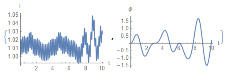
{Plot[sol.{1, 0}, {t, 0, 10}, AxesLabel -> {"t", "l"}], 
 Plot[sol.{0, 1}, {t, 0, 10}, AxesLabel -> {"t", "\[Phi]"}]}

fig1

Now I obtained my graphs.Thank you so much. :)

Anonymous User
Anonymous User
Posted 5 years ago

can i assume the initial problem didn't mention gravity and assumed orientation?

POSTED BY: Anonymous User
Posted 5 years ago

Thanks for reply.I found this code from hereThanks [@Hans Dolhaine ][1] for animate , but I can see just pendulum without spring and disc.How can add the disc and spring in this code?

z1 = {-R*W*Sin[W*t] + l'[t]*Sin[\[Phi][t]] + 
    l[t]*(\[Phi]'[t])*Cos[\[Phi][t]], 
   R*W*Cos[W*t] - l'[t]*Cos[\[Phi][t]] + 
    l[t]*(\[Phi]'[t])*Sin[\[Phi][t]]};

V = m*g*(R*Sin[W*t] - l[t]*Cos[\[Phi][t]]) + 1/2*k*(l[t] - l0)^2;
T = 1/2*m*z1.z1;
Lagrange = T - V;
eqs = D[D[Lagrange, \[Phi]'[t]], t] - D[Lagrange, \[Phi][t]];
eqs2 = D[D[Lagrange, l'[t]], t] - D[Lagrange, l[t]];

g = 9.7; m = 1; l0 = 1; k = 15; R = 2; W = Pi/2;
sol = NDSolve[{eqs == 0, eqs2 == 0, l[0] == l0, l'[0] == 0, 
    Derivative[1][\[Phi]][0] == 0, \[Phi][0] == 0}, {l[t], \[Phi][
     t]}, {t, 0, 30}];

z1a = z1 /. Flatten[sol /. a_[t] -> a];
Animate[Graphics[{Red, PointSize[.05], Point[z1a /. t -> tt]}, 
  Axes -> True, PlotRange -> {{-10, 10}, {-10, 10}}], {tt, 0, 30}]
POSTED BY: Ricardo Waste
Reply to this discussion
Community posts can be styled and formatted using the Markdown syntax.
Reply Preview
Attachments
Remove
or Discard

Group Abstract Group Abstract