Message Boards Message Boards

NDSolve for a heat differential equation with periodic boundary conditions?

I’m solving the heat differential equation in the steady state with a periodic temperature distribution along one side of the simulation volume (the notebook is attached).

Using NDSolve, I got very bad spatial resolution, i.e., the contour plot looks quite rough and not nice. Does anyone know how I can increase the resolution so that the plot looks nice? I suspect there is an option to increase the number of points.

I also would like to use periodic boundary conditions along the x-axis. So far I have terminated the simulation volume by Dirichlet boundary conditions after a finite number of periods, while the real-world temperature grating is entirely periodic along the x-direction. Any ideas?

Thanks, Markus

Attachments:
POSTED BY: Markus Schmidt
6 Replies

Hi Markus,

Take a look at the PeriodicBoundaryCondition>Scope>2D PDE Problems for an example on how to set up a PBC. Execute this code after you execute your code to see one possible implementation.

<< NDSolve`FEM`
\[CapitalOmega] = Rectangle[{0, 0}, {2 * \[CapitalLambda] , Lz}];
pde = -\!\(
\*SubsuperscriptBox[\(\[Del]\), \({x, z}\), \(2\)]\(u[x, z]\)\) == 0;
Subscript[\[CapitalGamma], D] = 
  DirichletCondition[
   u[x, z] == T0x[x], (z == 0) && 0 < x <= 2 * \[CapitalLambda] ];
Subscript[\[CapitalGamma], D2] = 
  DirichletCondition[
   u[x, z] == T0, (z == Lz) && 0 < x <= 2 * \[CapitalLambda]];
mesh = ToElementMesh[\[CapitalOmega], 
   "MaxBoundaryCellMeasure" -> 0.000001];
f = TranslationTransform[{2 * \[CapitalLambda], 0}];
pbc = PeriodicBoundaryCondition[u[x, z], x == 0, f];
ufun = NDSolveValue[{pde, pbc, Subscript[\[CapitalGamma], D], 
    Subscript[\[CapitalGamma], D2]}, u, {x, z} \[Element] mesh];
ContourPlot[ufun[x, z], {x, z} \[Element] mesh, MaxRecursion -> 4, 
 Contours -> 30, ColorFunction -> "BlueGreenYellow", 
 FrameStyle -> Directive[Black, Thickness[0.003]], 
 LabelStyle -> Directive[Black, 10], 
 FrameLabel -> {"x [m]", "z [m]"} ]
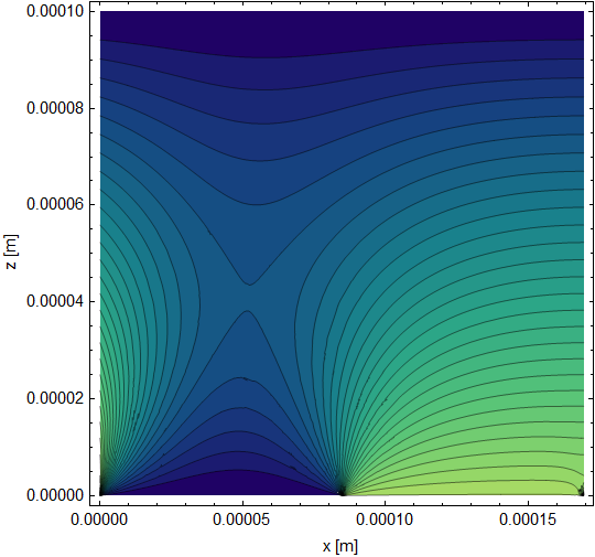
Periodic Solution

Compared to one period (the 5th to 6th) of your solution plotted using the following.

ContourPlot[
 us[x, z], {x, 5 2 \[CapitalLambda], 6 2 \[CapitalLambda]}, {z, 0, 
  Lz}, Contours -> 30, MaxRecursion -> 4, 
 ColorFunction -> "BlueGreenYellow", PlotPoints -> 200, 
 FrameStyle -> Directive[Black, Thickness[0.003]], 
 LabelStyle -> Directive[Black, 10], FrameLabel -> {"x [m]", "z [m]"}]
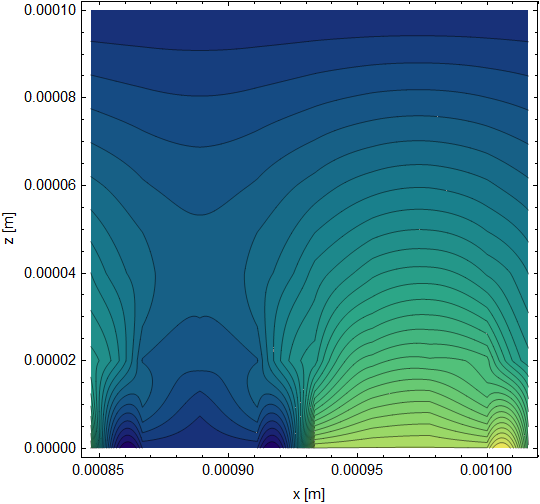
Markus Solution for One Period

Your current solution has some sharp features that I would not expect in a diffusion problem. In contrast, the periodic solution is smooth when you get away from boundary effects.

You can use the attached in case the formatting gets mucked up in the post due to special characters.

Also, MaxRecursion can be used to smooth out the plots, but it can take some time if the plot is complex.

Attachments:
POSTED BY: Tim Laska

Hi Tim.

This is really nice and exactly what I wanted, thanx.

Is there a simple way to plot multiple periods of the distribution in contourplot? Let's say I would like to plot five periods so that people can really see the periodic temperature distribution.

Best,

Markus

POSTED BY: Markus Schmidt

Hi Markus,

You could just define a function that shifts the contour plot and then seam them together with Show. For example:

cp[i_, n_] := 
  ContourPlot[
   ufun[x - 2*\[CapitalLambda] i, z], {x, 2*\[CapitalLambda]*i, 
    2*\[CapitalLambda]*(i + 1)}, {z, 0, Lz}, MaxRecursion -> 4, 
   Contours -> 30, ColorFunction -> "BlueGreenYellow", 
   FrameStyle -> Directive[Black, Thickness[0.003]], 
   LabelStyle -> Directive[Black, 10], 
   FrameLabel -> {"x [m]", "z [m]"} , 
   PlotRange -> {{0, 2 * \[CapitalLambda] * (n)}, {0, Lz}}];
nplts = 5;
Show[Table[cp[i, nplts], {i, 0, nplts - 1}]]

5 Contour Plots

Best regards and Happy New Year!

Tim

POSTED BY: Tim Laska

Great idea, thank you again.

Just as a side note: The solution shown in your plot is asymmetric along the x-axis, which is strange since it is there is nothing physical enforcing this. I shifted everything by lambda/2 in x-direction, and now it looks correct. enter image description here

Thanks again,

Markus

POSTED BY: Markus Schmidt

You're welcome Markus!

Good catch.

The following is an alternative way to create the stitched together graphic using Translate.

cplot = ContourPlot[
   ufun[x, z], {x, 0, 2*\[CapitalLambda]}, {z, 0, Lz}, 
   MaxRecursion -> 4, Contours -> 30, 
   ColorFunction -> "BlueGreenYellow" ];
n = 5;
Graphics[Table[
  Translate[First@cplot, {2 \[CapitalLambda] i, 0}], {i, 0, n}], 
 PlotRange -> {{0, 2 * \[CapitalLambda] * n}, {0, Lz}}, Frame -> True,
  FrameStyle -> Directive[Black, Thickness[0.003]], 
 LabelStyle -> Directive[Black, 10], FrameLabel -> {"x [m]", "z [m]"},
  AspectRatio -> 1]

Update

In the link that I provided, they actually show an example of how to stitch PBC problems together in the basic examples section. It probably is the simplest as shown below.

cplot = ContourPlot[
   ufun[x, z], {x, 0, 2*\[CapitalLambda]}, {z, 0, Lz}, 
   MaxRecursion -> 4, Contours -> 30, 
   ColorFunction -> "BlueGreenYellow", 
   FrameStyle -> Directive[Black, Thickness[0.003]], 
   LabelStyle -> Directive[Black, 10], 
   FrameLabel -> {"x [m]", "z [m]"} ];
n = 5;
Show[Table[
  MapAt[Translate[#, {2 \[CapitalLambda] i, 0}] &, cplot, 1], {i, 0, 
   n}], PlotRange -> All]

Attached is a corrected notebook include the shift noted by Markus.

Attachments:
POSTED BY: Tim Laska

Just as a remark:

... so that people can really see the periodic temperature distribution.

So how about this:

img = ImageCrop@
   ContourPlot[ufun[x, z], {x, z} \[Element] mesh, MaxRecursion -> 4, 
     Contours -> 30, ColorFunction -> "BlueGreenYellow",
    Frame -> False, PlotRangePadding -> 0, ImageSize -> 600];
ParametricPlot3D[{Cos[\[Phi]], Sin[\[Phi]], z}, {\[Phi], 0, 2 Pi}, {z,
   0, 0.0001}, PlotStyle -> Texture[img], Mesh -> None, 
 BoxRatios -> {1, 1, 1.5}, Ticks -> {None, None, Automatic}]

giving:

enter image description here

Regards -- Henrik

POSTED BY: Henrik Schachner
Reply to this discussion
Community posts can be styled and formatted using the Markdown syntax.
Reply Preview
Attachments
Remove
or Discard

Group Abstract Group Abstract