Hi Markus,
Take a look at the PeriodicBoundaryCondition>Scope>2D PDE Problems for an example on how to set up a PBC. Execute this code after you execute your code to see one possible implementation.
<< NDSolve`FEM`
\[CapitalOmega] = Rectangle[{0, 0}, {2 * \[CapitalLambda] , Lz}];
pde = -\!\(
\*SubsuperscriptBox[\(\[Del]\), \({x, z}\), \(2\)]\(u[x, z]\)\) == 0;
Subscript[\[CapitalGamma], D] =
DirichletCondition[
u[x, z] == T0x[x], (z == 0) && 0 < x <= 2 * \[CapitalLambda] ];
Subscript[\[CapitalGamma], D2] =
DirichletCondition[
u[x, z] == T0, (z == Lz) && 0 < x <= 2 * \[CapitalLambda]];
mesh = ToElementMesh[\[CapitalOmega],
"MaxBoundaryCellMeasure" -> 0.000001];
f = TranslationTransform[{2 * \[CapitalLambda], 0}];
pbc = PeriodicBoundaryCondition[u[x, z], x == 0, f];
ufun = NDSolveValue[{pde, pbc, Subscript[\[CapitalGamma], D],
Subscript[\[CapitalGamma], D2]}, u, {x, z} \[Element] mesh];
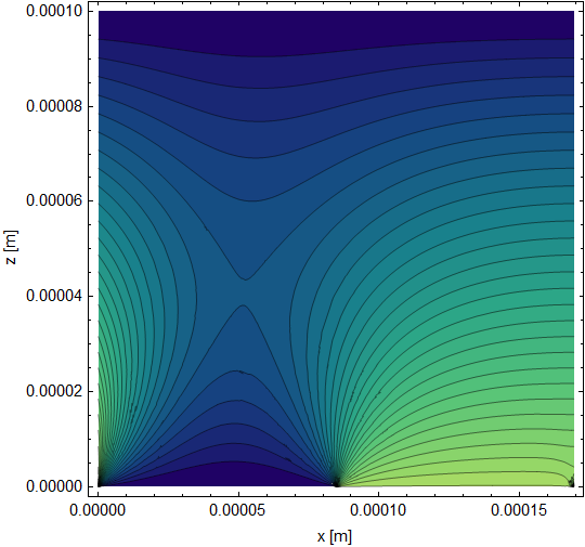
ContourPlot[ufun[x, z], {x, z} \[Element] mesh, MaxRecursion -> 4,
Contours -> 30, ColorFunction -> "BlueGreenYellow",
FrameStyle -> Directive[Black, Thickness[0.003]],
LabelStyle -> Directive[Black, 10],
FrameLabel -> {"x [m]", "z [m]"} ]
Compared to one period (the 5th to 6th) of your solution plotted using the following.
ContourPlot[
 us[x, z], {x, 5 2 \[CapitalLambda], 6 2 \[CapitalLambda]}, {z, 0,
  Lz}, Contours -> 30, MaxRecursion -> 4,
 ColorFunction -> "BlueGreenYellow", PlotPoints -> 200,
 FrameStyle -> Directive[Black, Thickness[0.003]],
 LabelStyle -> Directive[Black, 10], FrameLabel -> {"x [m]", "z [m]"}]
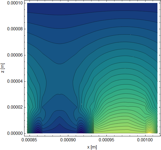
Your current solution has some sharp features that I would not expect in a diffusion problem. In contrast, the periodic solution is smooth when you get away from boundary effects.
You can use the attached in case the formatting gets mucked up in the post due to special characters.
Also, MaxRecursion can be used to smooth out the plots, but it can take some time if the plot is complex.
 Attachments:


