In the code below, a system of two first order non-linear differential equations are integrated. Would like some help understanding the result. There are two variables, z[t] and p[t]. The results appear to settle out with p[t] about 168 and z[t] about 0.99, and then after some time the system goes unstable and p begins to increase and z begins to oscillate.
My primary concern is the time range when p[t[ and z[t] appear to be constant. Plugging the values of z = 0.99 and p = 168 into the expression for dp/dt produces a value of about 2.4, so it is not clear why p[t] is staying constant during this period.
Below is the code.
dpRHS[z_, p_] := 4. (0.07 z Sqrt[600. - p] - 0.005 Sqrt[p p - 100.])

dzRHS[z_, p_] := Module[{dfVal, dzVal},
  dfVal = 4. (0.07 z Sqrt[600. - p] - 0.005 Sqrt[p p - 100.]);
  dzVal = -0.3 dfVal + 0.4 (170. - p);
  Piecewise[{{Max[0, dzVal], z <= 0.01}, {Min[0, dzVal], z >= 0.99}},
   dzVal]]

de = {p'[t] == dpRHS[z[t], p[t]], z'[t] == dzRHS[z[t], p[t]]};
ic = {p[0] == 140., z[0] == 0.5};
eqs = Flatten[{de, ic}]
tmax = 20;
{res, steps} =  Reap[solODE = NDSolve[eqs, {p, z}, {t, 0, tmax},   StepMonitor :> Sow[{t, z[t], p[t]}]]];

Plot[{p[t] /. solODE, 170}, {t, 0, tmax}, PlotRange -> {All, All},  PlotLabel -> "P[t]", PlotStyle -> {Sequence, {Red, Dashing[0.01]} }]
Plot[z[t] /. solODE, {t, 0, tmax}, PlotRange -> {All, All},  PlotLabel -> "Z[t]"]

(*inspect details of the numeric soluion*)
tzVals =  steps[[1, All, {1, 2}]];
tpVals  =  steps[[1, All, {1, 3}]];
tdpVals = {#[[1]],  dpRHS[#[[2]], #[[3]]  ]} & /@ steps[[1, All ]];

ListPlot[ tzVals , PlotRange -> {{12, 15}, All}, PlotLabel -> "Z[t]" ]
ListPlot[ tpVals , PlotRange -> {{12, 15}, {165, 175}},  PlotLabel -> "P[t]",
 Epilog -> {Red, Dashing[0.01], Line[{{0, 170}, {50, 170}}]}]
ListPlot[ tdpVals , PlotRange -> {{12, 15}, All},  PlotLabel -> "P'[t]   (computed from {z,p}" ]
Below are the plots of p[t] and z[t]. Which should p[t] increasing, but then stops increasing. 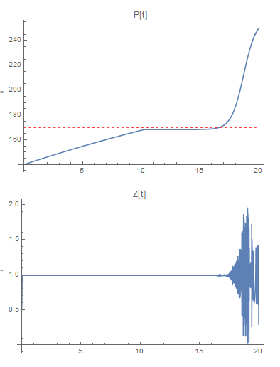
Note that for the time range from 10 to 15, the value of p appears to settle out near 168 and the value of z appears is first just below 1. Then at later times, the value of z becomes unstable. At the moment I am not too concerned about the instability (the coefficients can be changed to remove the instability.) At the moment I am concerned about the value of p for times between 10 and 15, when p appears to be constant; however, with a value of z around 0.99 and a value of p around 168, dp/dt should be around 2.4, so I would expect p to continue increasing. (Then when p > 170, p should begin to decrease. The system is intended to have a steady-state value of p = 170 and z = 0.58).
Additional information: this code was written to limit the value of z between 0 and 1. So the equation for the dz/dt is given as a piecewise function. When z gets close to 0, then dz/dt is only allowed to be greater than or equal to zero. When z gets close to 1, then dz/dt is only allowed to be less than or equal to zero.
Additional information, I used Reap/Sow, to investigate the individual steps that NDSolve was using. The results were similar to what one sees when inspecting the plot.
 Attachments:


