Hi Natasha,

You are probably approaching the limit of DSolve's ability to find an analytical solution (at least directly). You should consider a numerical solution for this problem.

If you are okay with a numerical solution, you can use the code below as a starting point.

tmax = 2/100;
ptmax = tmax/5;
eqn = D[u[x, t], t] == 100*D[u[x, t], {x, 2}] - 50*D[u[x, t], x];
ic = u[x, 0] == 50;
bc1 = u[0, t] == 50 + 20 Tanh[20000 t] ;
bc2 = (D[u[x, t], x] == 0) /. {x -> 1};
ndsol = NDSolveValue[{eqn, ic, bc1, bc2}, 
   u[x, t], {x, 0, 1}, {t, 0, tmax}, 
   Method -> {"MethodOfLines", 
     "SpatialDiscretization" -> {"TensorProductGrid", 
       "MinPoints" -> 50}}, MaxStepFraction -> 1/1000];
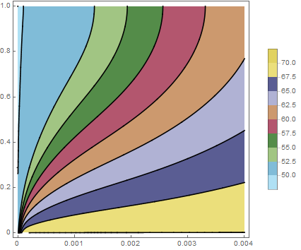
ContourPlot[ndsol, {t, 0.`, ptmax}, {x, 0.`, 1}, 
 PlotPoints -> {200, 200}, MaxRecursion -> 4, PlotTheme -> "Web", 
 ColorFunction -> ColorData["DarkBands"]]

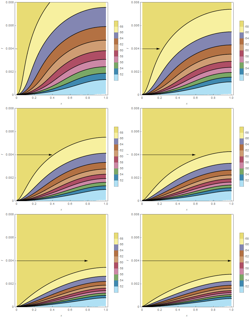
Note that I used a Tanh function to provide a rapidly rising "step" function so that the boundary and initial conditions were consistent. If you want to explore the effects of velocity on the solution, you could wrap the above (note that flipped the plot 90 degrees so it would flow left to right) into a Module like so.

condiff[v_] := Module[{tmax, ptmax, eqn, ic, bc1, bc2, ndsol, cp},
  tmax = 2/100;
  ptmax =  2 tmax/5;
  eqn = D[u[x, t], t] == 100*D[u[x, t], {x, 2}] - v*D[u[x, t], x];
  ic = u[x, 0] == 50;
  bc1 = u[0, t] == 50 + 20 Tanh[20000 t] ;
  bc2 = (D[u[x, t], x] == 0) /. {x -> 1};
  ndsol = 
   NDSolveValue[{eqn, ic, bc1, bc2}, u, {x, 0, 1}, {t, 0, tmax}, 
    Method -> {"MethodOfLines", 
      "SpatialDiscretization" -> {"TensorProductGrid", 
        "MinPoints" -> 2000}}, MaxStepFraction -> 1/1000];
  cp = ContourPlot[ndsol[x, t], {x, 0.`, 1}, {t, 0.`, ptmax}, 
    PlotRange -> {50, 70}, PlotPoints -> {50, 50}, MaxRecursion -> 4, 
    PlotTheme -> "Web", ColorFunction -> ColorData["DarkBands"], 
    FrameLabel -> Automatic];
  Show[{cp, Graphics[Arrow[{{0, 0.004}, {v/500, 0.004}}]]}]
  ]

Now, you can create an animation of velocities from 0 to 500 (it will take a while!).

imgs = Table[condiff[v], {v, 0, 500, 5}];
ListAnimate[imgs]

Thank you. I made the following changes,

eqn = D[u[x, t], t] == 100*D[u[x, t], {x, 2}];

and

asol[x_, t_] = dsol /. {\[Infinity] -> 30000} // Activate;

Plot[asol[0.5, t], {t, 1, 20}, PlotRange -> All]

However, the plot shows only a straight line at u = 70 (y-axis) from 0 to 20 seconds.I had expected the plot to start from 50 at t = 0 and reach 70 after the initial transient phase.

I'm not sure what's causing the problem. Any suggestions on how to get the right solution?

Thanks for the advice. I have changed the left boundary condition

bc1 = u[0, t] == 70;

sol = DSolveValue[{eqn, ic, bc1, bc2}, u[x, t], {x, t}]

gives,

70 + 2 Inactive[Sum][(
   40 E^(-225 \[Pi]^2 t (-1 + 2 K[1])^2)
     Sin[1/2 \[Pi] x (-1 + 2 K[1])])/(\[Pi] - 2 \[Pi] K[1]), {K[1], 
    1, \[Infinity]}]

Since the above solution is an infinite series, I am considering first 300 terms.

asol = sol /. {\[Infinity] -> 300}

Next, I am trying to plot the solution at x = 0.5 for time t= 1:20 using the following command

Plot(sol)

The above syntax isn't complete, I would like to ask for some help in specifying the syntax for plotting the above solution.

Solving for analytical solution of 1D transport equation

Many thanks for the response.I would like to if it is possible to view the complete expression of the analytical solution. I think the solution that is displayed after making the above-suggested change is the steady-state solution.

You need to write the no flux BC differently, but your specification returns a trivial result of 50 when corrected.

eqn = D[u[x, t], t] == D[u[x, t], {x, 2}];
ic = u[x, 0] == 50;
bc1 = u[0, t] == 50;
bc2 = (D[u[x, t], x] == 0) /. {x -> 1};
DSolve[{eqn, ic, bc1, bc2}, u[x, t], {x, t}] (* {{u[x, t] -> 50}} *)