You need to write the no flux BC differently, but your specification returns a trivial result of 50 when corrected.

eqn = D[u[x, t], t] == D[u[x, t], {x, 2}];
ic = u[x, 0] == 50;
bc1 = u[0, t] == 50;
bc2 = (D[u[x, t], x] == 0) /. {x -> 1};
DSolve[{eqn, ic, bc1, bc2}, u[x, t], {x, t}] (* {{u[x, t] -> 50}} *)

Solving for analytical solution of 1D transport equation

I think that you will need to rethink your specification. Right now, your initial condition says that the temperature is 50 everywhere. Your first boundary condition says that the temperature at the boundary is 50. Your second boundary conditions says that the system is insulated at the end. How can the system change from the value of 50 everywhere?

Look at the DSolveValue>Applications>Classical Partial Differential Equations for an example how to do this.

eqn = D[u[x, t], t] == D[u[x, t], {x, 2}];
ic = u[x, 0] == 50;
bc1 = u[0, t] == 70;
bc2 = (D[u[x, t], x] == 0) /. {x -> 1};
dsol = DSolveValue[{eqn, ic, bc1, bc2}, 
    u[x, t], {x, t}] /. {K[1] -> m};
asol[x_, t_] = dsol /. {\[Infinity] -> 300} // Activate;
Plot[asol[0.5, t], {t, 1, 20}, PlotRange -> All]

Note that a value of 300 causes a warning about the value being too small.

Hi Natasha,

Your diffusion coefficient is huge and that implies that the system responds very quickly. To see this response, you will need to look at times much closer to 0 and not begin at $t=1$. You probably do not need many terms to capture the response.

eqn = D[u[x, t], t] == 100 D[u[x, t], {x, 2}];
ic = u[x, 0] == 50;
bc1 = u[0, t] == 70;
bc2 = (D[u[x, t], x] == 0) /. {x -> 1};
dsol = DSolveValue[{eqn, ic, bc1, bc2}, 
    u[x, t], {x, t}] /. {K[1] -> m};
asol5[x_, t_] = dsol /. {\[Infinity] -> 5} // Activate;
asol10[x_, t_] = dsol /. {\[Infinity] -> 300} // Activate;
Plot[{asol5[0.5, t], asol10[0.5, t]}, {t, 0, 0.001}, PlotRange -> All]

Hi Natasha,

You are probably approaching the limit of DSolve's ability to find an analytical solution (at least directly). You should consider a numerical solution for this problem.

If you are okay with a numerical solution, you can use the code below as a starting point.

tmax = 2/100;
ptmax = tmax/5;
eqn = D[u[x, t], t] == 100*D[u[x, t], {x, 2}] - 50*D[u[x, t], x];
ic = u[x, 0] == 50;
bc1 = u[0, t] == 50 + 20 Tanh[20000 t] ;
bc2 = (D[u[x, t], x] == 0) /. {x -> 1};
ndsol = NDSolveValue[{eqn, ic, bc1, bc2}, 
   u[x, t], {x, 0, 1}, {t, 0, tmax}, 
   Method -> {"MethodOfLines", 
     "SpatialDiscretization" -> {"TensorProductGrid", 
       "MinPoints" -> 50}}, MaxStepFraction -> 1/1000];
ContourPlot[ndsol, {t, 0.`, ptmax}, {x, 0.`, 1}, 
 PlotPoints -> {200, 200}, MaxRecursion -> 4, PlotTheme -> "Web", 
 ColorFunction -> ColorData["DarkBands"]]

Note that I used a Tanh function to provide a rapidly rising "step" function so that the boundary and initial conditions were consistent. If you want to explore the effects of velocity on the solution, you could wrap the above (note that flipped the plot 90 degrees so it would flow left to right) into a Module like so.

condiff[v_] := Module[{tmax, ptmax, eqn, ic, bc1, bc2, ndsol, cp},
  tmax = 2/100;
  ptmax =  2 tmax/5;
  eqn = D[u[x, t], t] == 100*D[u[x, t], {x, 2}] - v*D[u[x, t], x];
  ic = u[x, 0] == 50;
  bc1 = u[0, t] == 50 + 20 Tanh[20000 t] ;
  bc2 = (D[u[x, t], x] == 0) /. {x -> 1};
  ndsol = 
   NDSolveValue[{eqn, ic, bc1, bc2}, u, {x, 0, 1}, {t, 0, tmax}, 
    Method -> {"MethodOfLines", 
      "SpatialDiscretization" -> {"TensorProductGrid", 
        "MinPoints" -> 2000}}, MaxStepFraction -> 1/1000];
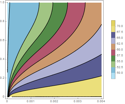
  cp = ContourPlot[ndsol[x, t], {x, 0.`, 1}, {t, 0.`, ptmax}, 
    PlotRange -> {50, 70}, PlotPoints -> {50, 50}, MaxRecursion -> 4, 
    PlotTheme -> "Web", ColorFunction -> ColorData["DarkBands"], 
    FrameLabel -> Automatic];
  Show[{cp, Graphics[Arrow[{{0, 0.004}, {v/500, 0.004}}]]}]
  ]

Now, you can create an animation of velocities from 0 to 500 (it will take a while!).

imgs = Table[condiff[v], {v, 0, 500, 5}];
ListAnimate[imgs]