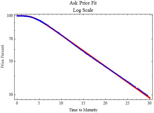
I have developed a model for fitting zero-coupon Treasury bonds to price data. It can take data from a Wall Street Journal public page or data from a brokerage account web page may be pasted into the Mathematica notebook and analyzed. Here is an example of a recent fit.

The blue dots are data points and the red line the fit. Below are the parameter statistics.

The model is based on the survival function of a probability distribution which is the sum of an exponential distribution random variable and a gamma distribution random variable. The formula is obtained as follows:
(*I haven't been able to do this with Integrate[].**)
(*For fitting the price model the constraint r0 != r1 has to be added**)
td = TransformedDistribution[
x + y, {x \[Distributed] ExponentialDistribution[r0],
y \[Distributed] GammaDistribution[k, 1/r1]}];
SurvivalFunction[td, t] // FullSimplify

The model is then fit with NonlinearModelFit[] using some initial parameter starting points. The model is described in detail at the website below.
http://pages.suddenlink.net/rhr/fin07/TreasuryZeroes.htmlOr the Mathematica notebook containing all the functions can be opened with the following line of code:
NotebookPut@Import["http://pages.suddenlink.net/rhr/fin07/TreasuryZeroes.nb"];
Why this should work so well is something of a mystery. Is it another case of "
The Unreasonable Effectiveness of Mathematics in the Natural Sciences," or does it point to some underlying truth? Comments and ideas will be appreciated