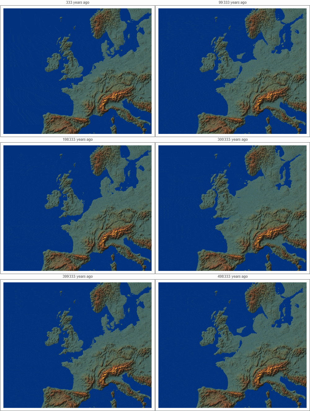
The Pleistocene Epoch ended 12,000 years ago, making way for the Holocene Epoch which continues to today. During the peak of the last glacial episode, tremendous amounts of water was locked away in the glaciers which caused sea levels to drop. As the Pleistocene came to a close, glaciers from the last glacial episode were melted which caused the sea levels to rise. The following exploration uses data from De Boer, B., R.S.W. Van de Wal, R. Bintanja, L.J. Lourens and E. Tuenter, "Cenozoic global ice-volume and temperature simulations with 1-D ice-sheet models forced by benthic d18O records", Annals of Glaciology, 51 (55), 23-33, 2010.

sealeveldata = Transpose[
  QuantityMagnitude[
   Normal[Values[
     ResourceData[
       "Sea Level and Temperatures Over the Last 40 Million \
                Years"][{"TimeBeforePresent", "SeaLevel"}]]]]];

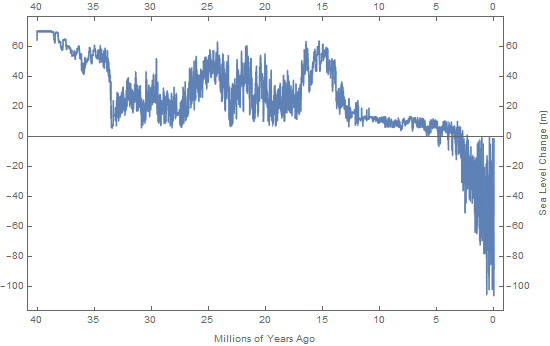
Over the last 40 million years, the global temperatures and sea levels have changed. Prior to 2.5 million years ago, the global sea level tended to be higher than it is today as global temperatures were warmer.

ListPlot[sealeveldata, Joined -> True, Frame -> True, PlotRange -> All,
  FrameLabel -> {{None, 
    "Sea Level Change (m)"}, {"Millions of Years Ago", None}}, 
 FrameTicks -> {{Table[{i, i}, {i, -140, 80, 20}], 
    Table[{i, i}, {i, -140, 80, 
      20}]}, {Table[{i, -i/1000000}, {i, -40000000, 0, 5000000}], 
    Table[{i, -i/1000000}, {i, -40000000, 0, 5000000}]}}, 
 ImageSize -> 550]

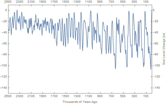
Starting about 2.5 million years ago, as the Pleistocene Epoch was starting, global temperatures started to drop and permanent ice started to form at the poles. We entered an ice age. During the Pleistocene, temperatures varied wildly and glaciers advanced and retreated in many pulses. Today, there is still permanent ice at the poles so we are still in an ice age. But we are between cold pulses, so we are in an interglacial period within the current ice age.

ListPlot[sealeveldata, Joined -> True, Frame -> True, 
 PlotRange -> {{-2500000, 0}, {-150, 10}}, 
 FrameTicks -> {{Table[{i, i}, {i, -140, 0, 20}], 
    Table[{i, i}, {i, -140, 0, 
      20}]}, {Table[{i, -i/1000}, {i, -2500000, 0, 200000}], 
    Table[{i, -i/1000}, {i, -2500000, 0, 200000}]}}, 
 FrameLabel -> {{None, 
    "Sea Level Change (m)"}, {"Thousands of Years Ago", None}}, 
 ImageSize -> 550]

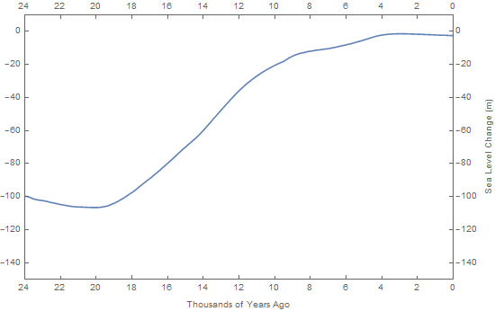
We can focus in on the peak of the last glacial episode to find the lowest sea level which happened about 20,000 years ago, when the glaciers locked up a large amount of water from the oceans.

ListPlot[sealeveldata, Joined -> True, Frame -> True, 
 PlotRange -> {{-24000, 0}, {-150, 10}}, 
 FrameTicks -> {{Table[{i, i}, {i, -140, 0, 20}], 
    Table[{i, i}, {i, -140, 0, 20}]}, {Table[{i, -i/1000}, {i, -24000,
       0, 2000}], Table[{i, -i/1000}, {i, -24000, 0, 2000}]}}, 
 FrameLabel -> {{None, 
    "Sea Level Change (m)"}, {"Thousands of Years Ago", None}}, 
 ImageSize -> 550]

For more continuous coverage, we can interpolate the data.

seaint = Interpolation[sealeveldata, InterpolationOrder -> 1];

To see the effects that changing sea levels had on the coast of the U.K. and Europe, first we need to obtain the elevation data using GeoElevationData. The following form works nicely using the forthcoming version 12:

data = GeoElevationData[
   Entity["City", {"London", "GreaterLondon", "UnitedKingdom"}], 
   GeoRange -> Quantity[800, "Miles"], GeoProjection -> Automatic, 
   UnitSystem -> "Metric"];

You can get similar results from 11.3 and earlier using the following definition:

data = GeoElevationData[
   GeoDisk[Entity[
     "City", {"London", "GreaterLondon", "UnitedKingdom"}], 
    Quantity[800, "Miles"]], UnitSystem -> "Metric"];

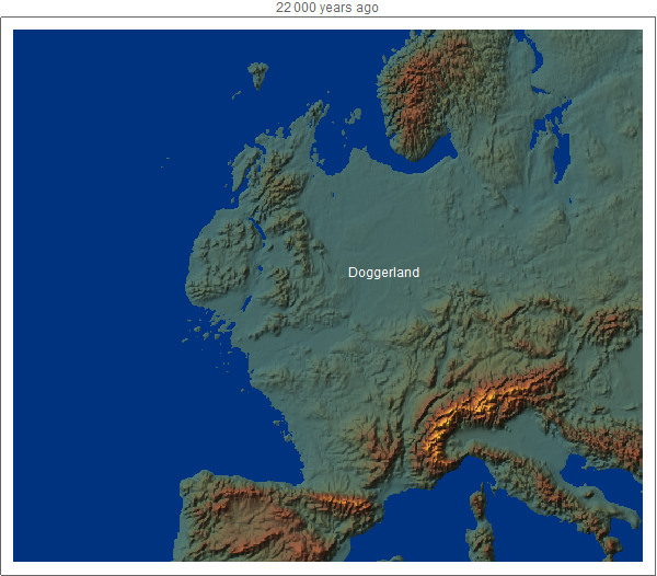
The following variations all use the data generated from version 12. At the greatest extent of the glacial event, the U.K. was connected to mainland Europe. The connecting land is often referred to as Doggerland. As long as the U.K. and Europe were connected, hunter-gatherers were able to move back and forth.

With[{ybp = -22000},
 ReliefPlot[Reverse[data], 
  PlotRange -> {Full, Full, {seaint[ybp], All}}, ImageSize -> 600, 
  ColorFunction -> "FallColors", ClippingStyle -> RGBColor[0, .2, .5],
   PerformanceGoal -> "Quality", 
  PlotLabel -> Row[{-Round[ybp], " years ago"}], 
  Epilog -> {Text[Style["Doggerland", 12, White], {320, 250}]}, 
  FrameTicks -> All]]

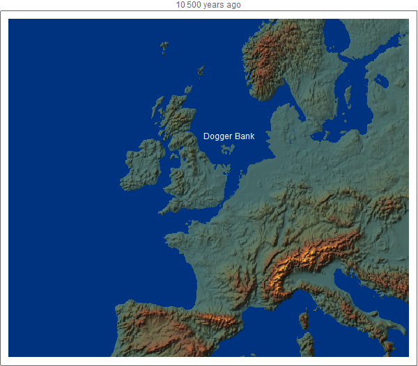
By about 10,500 years ago (8,500 BCE) sea levels rose to the point that the U.K. had basically separated from the European mainland. A small uprise known as the Dogger Bank was still exposed as an island.

With[{ybp = -10500},
 ReliefPlot[Reverse[data], 
  PlotRange -> {Full, Full, {seaint[ybp], All}}, ImageSize -> 600, 
  ColorFunction -> "FallColors", ClippingStyle -> RGBColor[0, .2, .5],
   PerformanceGoal -> "Quality", 
  PlotLabel -> Row[{-Round[ybp], " years ago"}], 
  Epilog -> {Text[Style["Dogger Bank", 12, White], {300, 300}]}]]

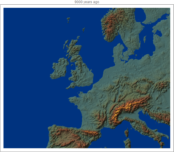
By 9,000 years ago (7,000 BCE), the Dogger Bank had also submerged.

With[{ybp = -9000},
 ReliefPlot[Reverse[data], 
  PlotRange -> {Full, Full, {seaint[ybp], All}}, ImageSize -> 600, 
  ColorFunction -> "FallColors", ClippingStyle -> RGBColor[0, .2, .5],
   PerformanceGoal -> "Quality", 
  PlotLabel -> Row[{-Round[ybp], " years ago"}]]]

An animated version can be created as well. Here is a link I created showing the variation in sea level over the last 500,000 years. Time will tell if we will enter a new glacial period and see the glaciers once again advance as they have many times in the last 2.5 million years.