One of my longstanding research interests in numerical analysis has been the family of "simultaneous iteration" methods for finding polynomial roots. (See e.g. McNamee's book for a comprehensive survey.) Briefly put, these are modified Newton-Raphson methods that allow one to find the roots of a polynomial all at once, as opposed to finding them one at a time and "deflating".

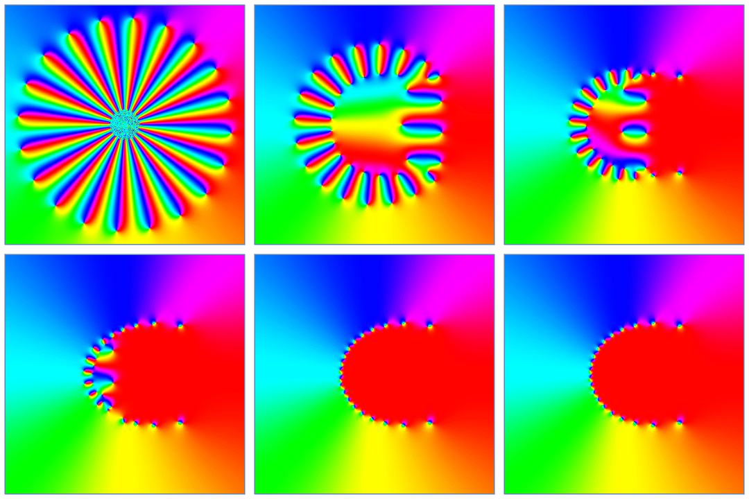
I had the idea to visualize how these algorithms gradually proceed from initial approximations to the roots, up to convergence. After a number of experiments, I settled on using domain coloring for visualization. I have found that the logarithmic derivatives of polynomials gave particularly striking plots.

For this post, I have used the scaled exponential sum of degree 20:

$$\frac{20!}{20^{20}}\sum_{k=0}^{20}\frac{(20z)^k}{k!}$$

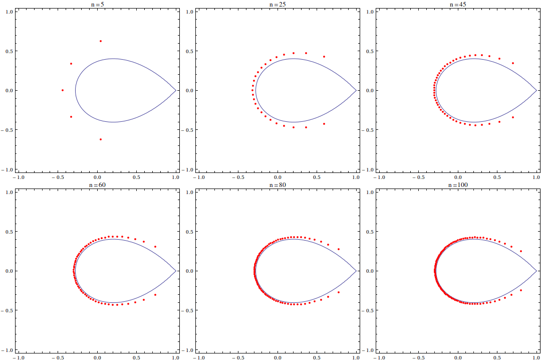
as the example polynomial whose roots we want to see. It is known that the zeroes of this polynomial asymptotically approach the so-called Szeg? curve as the polynomial degree goes to infinity.

expPoly[x_] = With[{n = 20}, Sum[(n! (n x)^k)/(k! n^n), {k, 0, n}]]

I will now look at two of the most popular simultaneous iteration methods. The first one is the (Weierstrass-)Durand-Kerner method,

$$x_i^{(k+1)}=x_i^{(k)}-\frac{p(x_i^{(k)})}{\prod\limits_{j\neq i} (x_i^{(k)}-x_j^{(k)})},\qquad i=1\dots n;\; k=0,1,\dots$$

which is (typically) quadratically convergent. (Note that in simultaneous iteration methods, the polynomials are always assumed to be monic (i.e., unit leading coefficient).)

Implementing the iteration is easy using FixedPointList[]. As is customary with these methods, we use as a starting approximation points equispaced around the unit circle, and slightly rotated:

ptsdk = FixedPointList[# - expPoly[#]/Table[Apply[Times, #[[k]] - Delete[#, k]],
                                            {k, Length[#]}] &,
                       N[Exp[2 ? I Range[0, 19]/20 - I ?/40]], 40,
                       SameTest -> (EuclideanDistance[##] < 1.*^-6 &)];

I use a loose convergence criterion that is good enough for visualization purposes.

For the domain coloring plot, I will use a slightly modified version of the DLMF color scheme, based on an idea of Quilez.

DLMFPhaseColor[u_, s_:1, b_:1] := Module[{rgb},
          rgb = Clip[{1, -1, -1} Abs[{8, 4, 8} Mod[u/(2 ?), 1] -
                     {9, 3, 11}/2] + {-3, 3, 5}/2, {0, 1}];
          rgb = (3 - 2 rgb) rgb^2;
          Apply[RGBColor, b (1 + s (rgb - 1))]]

I then use a simplified version of code originally written by user Heike on Mathematica Stack Exchange:

dcdk = RegionPlot[True, {x, -9/8, 9/8}, {y, -9/8, 9/8}, 
                  ColorFunction ->
                  Function[{x, y}, DLMFPhaseColor[Arg[Total[1/(x + I y - #)]]]], 
                  ColorFunctionScaling -> False, Frame -> False, 
                  PlotPoints -> 405] & /@ ptsdk;

(This takes some time, due to the high PlotPoints setting.)

We can now see an animation:

ListAnimate[dcdk]

The other method I will be looking at in this post is the (typically) cubically convergent Ehrlich-Aberth(-Maehly) method,

$$x_i^{(k+1)}=x_i^{(k)}-\frac{\tfrac{p(x_i^{(k)})}{p^\prime(x_i^{(k)})}}{1-\tfrac{p(x_i^{(k)})}{p^\prime(x_i^{(k)})}\sum\limits_{j\neq i} \tfrac1{x_i^{(k)}-x_j^{(k)}}},\qquad i=1\dots n;\; k=0,1,\dots$$

which is also one of the methods available in Mathematica's NSolve[]/NRoots[].

Unfortunately, I have no way to get the iterates generated by NSolve[], so I had to reimplement the method myself. We can use essentially the same code as was used for Durand-Kerner, with a few changes:

ptsea = FixedPointList[With[{ld = expPoly[#]/expPoly'[#]},
                            # - ld/(1 - ld Table[Tr[1/(#[[k]] - Delete[#, k])],
                                                 {k, Length[#]}])] &,
                       N[Exp[2 ? I Range[0, 19]/20 - I ?/40]], 40,
                       SameTest -> (EuclideanDistance[##] < 1.*^-6 &)];

dcea = RegionPlot[True, {x, -9/8, 9/8}, {y, -9/8, 9/8}, 
                  ColorFunction ->
                  Function[{x, y}, DLMFPhaseColor[Arg[Total[1/(x + I y - #)]]]], 
                  ColorFunctionScaling -> False, Frame -> False, 
                  PlotPoints -> 405] & /@ ptsea;

ListAnimate[dcea]

It would be interesting to use this visualization technique on other polynomials with interesting root structure, as well as other simultaneous iteration methods.