I recently wanted to learn more about recurrent neural networks (RNNs) and how to use them for regression problems. In particular, I wanted to try and combine RNNs with the ideas for Bayesian error bar estimation I discussed in my blog/community posts a while back:
https://blog.wolfram.com/2018/05/31/how-optimistic-do-you-want-to-be-bayesian-neural-network-regression-with-prediction-errors/ https://community.wolfram.com/groups/-/m/t/1319745
I also found the found the following answer on StackExchange about sequence learning with SequenceAttentionLayer, which helped me quite a bit to understand how to use to use these layers: https://mathematica.stackexchange.com/a/143672/43522
With those resources in hand, I wanted to give time-series regression a shot.
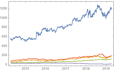
First, let's use FinancialData as an easy source of a test dataset. Here I download 5 years of data from 5 different indices and turn them into a regularly sampled matrix of vectors and then split the dataset into 80/20% training/test data:
indices = {"GOOGL", "AS:ASML", "MSFT", "AAPL", "GE"};
data = FinancialData[indices, {Today - 5 Quantity[1, "Years"], Today}];
DateListPlot[data]
With[{
   matrix = N@Normal[
       TimeSeriesRescale[
        TimeSeriesResample[TimeSeriesThread[Identity, TimeSeries /@ data]], {0, Max[Length /@ data] - 1}]
    ][[All, 2]]
  },
  {fe, data} = FeatureExtraction[matrix,  "StandardizedVector", {"ExtractorFunction", "ExtractedFeatures"}]
  ];
{trainingData, testData} = TakeDrop[data, Round[0.8*Length[data]]];
Dimensions /@ {trainingData, testData}

Next, we define a function that can generate training data for the network from the data matrix we just made:
Clear[genFun];
genFun[data_, { seqLengthIn_, seqLengthout_, offset_}] := With[{
    dim = Dimensions[data][[2]],
    max = Max[1, Length[data] - seqLengthout - offset - seqLengthIn - 2]
    },
   Function[
    With[{ri = RandomInteger[{1, max}, #BatchSize]},
     <|
      "Input" -> Function[data[[# ;; # + seqLengthIn - 1]]] /@ ri,
      "Target" -> Join[
        ConstantArray[{ConstantArray[0., dim]}, #BatchSize],
        Function[With[{j = # + offset + seqLengthIn - 1},   data[[j ;; j + seqLengthout - 1]]]] /@ ri,
        2
        ]
      |>]]];
Each time the function is called, it generates a batch of sequences that will be used as training input and target sequences that the network should try to learn and reproduce, but the targets are prepended with a blank start-of-sequence vector:
Dimensions /@ genFun[data, {10, 6, 1}][<|"BatchSize" -> 3|>]
Out[72]= <|"Input" -> {3, 10, 5}, "Target" -> {3, 7, 5}|>
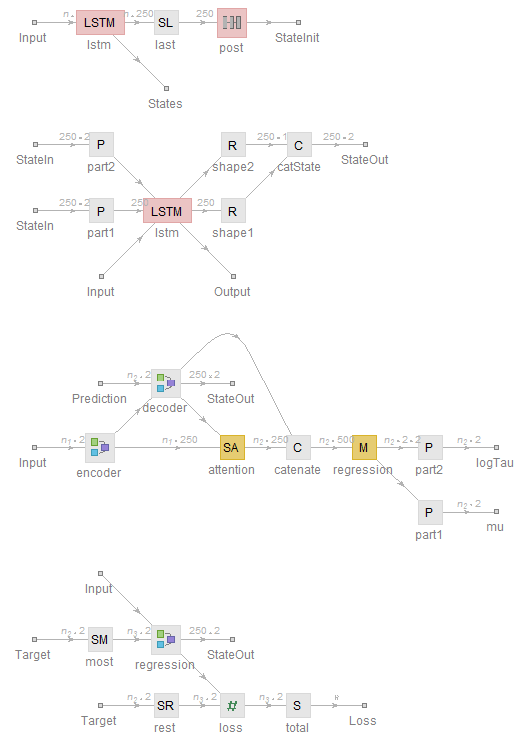
Next we put together our neural network:
Clear[encoderNetAttend, decoderNet, lossLayer, trainingNetAttention];
encoderNetAttend[n_, dropout_] := NetGraph[<|
    "lstm" -> LongShortTermMemoryLayer[n, "Dropout" -> dropout],
    "last" -> SequenceLastLayer[],
    "post" ->
     NetChain[{LinearLayer[n], ElementwiseLayer["SELU"],
       DropoutLayer[], LinearLayer[]}]
    |>,
   {"lstm" -> "last" -> "post" -> NetPort["StateInit"],  "lstm" -> NetPort["States"]}
   ];
decoderNet[n_, dropout_] := NetGraph[
   <|
    "part1" -> PartLayer[{All, 1}], "part2" -> PartLayer[{All, 2}],
    "lstm" -> LongShortTermMemoryLayer[n, "Dropout" -> dropout],
    "shape1" -> ReshapeLayer[{n, 1}],  "shape2" -> ReshapeLayer[{n, 1}], "catState" -> CatenateLayer[2]
    |>,
   {
    NetPort["Input"] -> NetPort["lstm", "Input"],
    NetPort["lstm", "Output"] -> NetPort["Output"],
    NetPort["StateIn"] -> "part1" -> NetPort["lstm", "State"],
    NetPort["StateIn"] -> "part2" -> NetPort["lstm", "CellState"],
    NetPort["lstm", "State"] -> "shape1",  NetPort["lstm", "CellState"] -> "shape2",
    {"shape1", "shape2"} -> "catState" -> NetPort["StateOut"]
    },
   "StateIn" -> {n, 2}
   ];
lossLayer["LogPrecision"] =  ThreadingLayer@Function[{yObserved, yPredicted, logPrecision},
    (yPredicted - yObserved)^2*Exp[logPrecision] - logPrecision
    ];
regressionNet[n_, dimIn_, dropout : _?NumericQ : 0.5] :=
  NetInitialize@NetGraph[
    <|
     "encoder" -> encoderNetAttend[n, dropout],
     "decoder" -> decoderNet[n, dropout],
     "attention" -> SequenceAttentionLayer["Bilinear"],
     "catenate" -> CatenateLayer[2],
     "regression" -> NetMapOperator[LinearLayer[{2, dimIn}]],
     "part1" -> PartLayer[{All, 1}], "part2" -> PartLayer[{All, 2}]
     |>,
    {
     NetPort["Input"] -> "encoder",
     NetPort["encoder", "StateInit"] -> NetPort["decoder", "StateIn"],
      NetPort["encoder", "States"] -> NetPort["attention", "Input"],
     NetPort["Prediction"] -> NetPort["decoder", "Input"],
     NetPort[{"decoder", "Output"}] ->
      NetPort["attention", "Query"], {"decoder", "attention"} ->
      "catenate" -> "regression",
     "regression" -> "part1" -> NetPort["mu"],
     "regression" -> "part2" -> NetPort["logTau"]
     },
    "Input" -> {"Varying", dimIn},
    "Prediction" -> {"Varying", dimIn}
    ];
trainingNetAttention[n_, dimIn_, dropout : _?NumericQ : 0.5] := NetInitialize@NetGraph[
    <|
     "regression" -> regressionNet[n, dimIn, dropout],
     "loss" -> lossLayer["LogPrecision"],
     "total" -> SummationLayer[],  "most" -> SequenceMostLayer[],  "rest" -> SequenceRestLayer[]
     |>,
    {
     NetPort["Input"] -> NetPort["regression", "Input"],
     NetPort["Target"] ->  "most" -> NetPort["regression", "Prediction"],
     NetPort["Target"] -> "rest",
     {"rest", NetPort["regression", "mu"],  NetPort["regression", "logTau"]} -> "loss" -> "total" -> NetPort["Loss"]
     },
    "Input" -> {"Varying", dimIn},
    "Target" -> {"Varying", dimIn}
    ];
nHidden = 250;
pDrop = 0.25;
NetInformation[encoderNetAttend[nHidden, pDrop], "SummaryGraphic"]
NetInformation[decoderNet[nHidden, pDrop], "SummaryGraphic"]
NetInformation[regressionNet[nHidden, 2, 0.25], "SummaryGraphic"]
NetInformation[ trainingNetAttention[nHidden, 2, 0.25], "SummaryGraphic"]

The idea here is that the encoder produces a state vector that the decoder uses to start making predictions. The decoder, in turn, accepts the networks' own predictions to iteratively crank out the next one. During the training, though, we don't have the actual predictions from the network, so instead we feed in the sequence of actual target values and offset the target sequence at the loss layer by one with a SequenceRest layer. This is called teacher forcing.
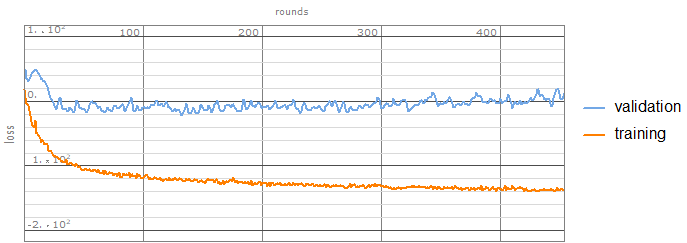
Time to train the network:
seqConfig = {15, 7, 1};
trainedTrainObject = NetTrain[
   trainingNetAttention[nHidden, Length[indices], pDrop],
   genFun[trainingData, seqConfig],
   All,
   TargetDevice -> "GPU",  LossFunction -> "Loss",
   TimeGoal -> 30*60, BatchSize -> 200,
   ValidationSet -> genFun[testData, seqConfig][<|"BatchSize" -> 200|>]
   ];
trainedNet = trainedTrainObject["TrainedNet"];
trainedTrainObject["EvolutionPlots"]

To make predictions, the network needs to eat its own results iteratively, which we can do with a NestList
makePredictorFunction[trainedNet_, evaluationMode : ("Test" | "Train") : "Test", device : ("CPU" | "GPU") : "CPU"] := With[{
   dim = Last@NetExtract[trainedNet, {"Input"}],
   encoder = NetExtract[trainedNet, {"regression", "encoder"}],
   regressionNet =
    NetDelete[NetExtract[trainedNet, "regression"], "encoder"]
   },
  Function[{input, n},
   Module[{
     encodedInput = encoder[input, NetEvaluationMode -> evaluationMode, TargetDevice -> device],
     vectorInputQ = Depth[input] === 4,
     length = Length[input],
     reshape
     },
    reshape = If[vectorInputQ, ConstantArray[#, Length[input]] &, Identity];
    GeneralUtilities`AssociationTranspose@NestList[
       regressionNet[
         <|"Input" -> encodedInput["States"], "Prediction" -> #mu, "StateIn" -> #StateOut|>,
          NetEvaluationMode -> evaluationMode,
         TargetDevice -> device] &,
       <|
        "mu" -> reshape@{ConstantArray[0, dim]},
        "StateOut" -> encodedInput["StateInit"]
        |>,
       n
       ][[2 ;;, {"mu", "logTau"}, If[vectorInputQ, All, Unevaluated[Sequence[]]], 1]]
    ]
   ]
  ];
For example, we can predict 5 steps ahead based on 30 points of historical data:
predictor = makePredictorFunction[trainedNet, "Train", "CPU"];
Dimensions /@ predictor[data[[;; 30]], 7]

Out[299]= <|"mu" -> {7, 5}, "logTau" -> {7, 5}|>
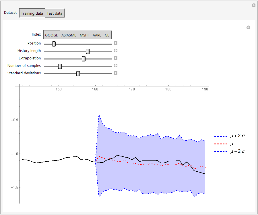
Here's a manipulate to visualize the predictions against the actual data. We sample the network several times to get a sense of the uncertainty from the training weights and combine that uncertainty with the variance predicted by the network:
Manipulate[
 Manipulate[
  Quiet@With[{
     predictions = Dot[
       {{1., 1.}, {1., 0.}, {1., -1.}},
       {Mean[#mu],
          nstdev*Sqrt[Variance[#mu] + Mean[Exp[-#logTau]]]} &@Map[
          Transpose,
          predictor[Table[dat[[Max[1, n - t] ;; UpTo[n]]], s], l]
          ][[{"mu", "logTau"}, All, All, index]]
       ],
     trueData = ListPlot[
       MapIndexed[{First[#2] + Max[1, n - t] - 1, #1} &,
        Flatten[dat[[Max[1, n - t] ;; UpTo[n + l], index]]]
        ],
       Joined -> True,
       PlotStyle -> Black
       ]
     },
    Show[
     ListPlot[
      Thread@Legended[
        MapIndexed[
           {First[#2] + Max[1, n - t] - 1, #1} &,
           Flatten[{
             dat[[Max[1, n - t] ;; UpTo[n], index]],
              #
             }]
           ] & /@ predictions,
        {StringForm["\[Mu] + `1` \[Sigma]", Dynamic[nstdev]],
         "\[Mu]", StringForm["\[Mu] - `1` \[Sigma]", Dynamic[nstdev]]}
        ],
      Joined -> True,
      PlotStyle -> (Directive[#, Dashed] & /@ {Blue, Red, Blue}),
      ImageSize -> 500,
      Filling -> {1 -> {2}, 3 -> {2}}
      ],
     trueData,
     ImageSize -> Large,
     PlotRange -> All
     ]
    ],
  {{index, 1, "Index"}, Thread[Range[Length[indices]] -> indices]},
  {{n, Round[Length[dat]/10], "Position"}, 1, Length[dat], 1},
  {{t, 20, "History length"}, 1, 30, 1},
  {{l, 30, "Extrapolation"}, 1, 50, 1},
  {{s, 5, "Number of samples"}, 1, 20, 1},
  {{nstdev, 2, "Standard deviations"}, 0, 4, 0.1},
  Paneled -> False,
  ContinuousAction -> True,
  TrackedSymbols :> {index, n, t, l, s, nstdev},
  SynchronousInitialization -> False
  ],
 {{dat, trainingData, "Dataset"}, {trainingData -> "Training data",
   testData -> "Test data"}},
 TrackedSymbols :> {dat},
 SynchronousInitialization -> False
 ]

The results on the validation set do not look great, but the comparison between the first 4 years of the data and the last one may not be fair. Or it may simply be necessary to involve many more indices before it becomes feasible to do extrapolations of this type. At any rate, I hope that this code is useful to other users here! I will probably tweak bits of code here and there over the next few days and maybe add more commentary, so be sure to check back occasionally if you're interested.
Update Some of the code needed to be updated slightly to work in the recently released Mathematica V12. The SequenceAttentionLayer is being phased out, but still works (see the "Properties & Relations" documentation for AttentionLayer for information about how to replace SequenceAttentionLayer with AttentionLayer). The financial data also needed a few more processing steps in V12 before it can be used. Please see the attached notebook for the V12 version of the code.
Update 2 (10 June 2019) I attached another notebook with code for a neural network that does not use teacher forcing but instead feeds its own predictions back into itself during training. This makes sure that the network is trained in exactly the same way as it is used afterwards. This also removes the need to use a NestList afterwards to generate the predictions. Training the network becomes trickier, though, and you need to experiment more with learning rate multipliers and gradient clipping to get convergence.
Update 3 (13 July 2020) I just updated the notebooks to make sure that all the code works correctly in Mathematica V12.1
To make this code work, you may need to update your neural network paclet first by evaluating:
PacletUpdate["NeuralNetworks"]
 Attachments: