Hi,
Is it possible to draw figures like below plots in the Mathematica? 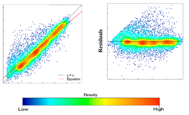
data1 = {9.186654398965594`, 11.32413825912701`, 12.999492089337714`,
10.948577055056163`, 10.466966636206493`, 10.032664245063756`,
11.100934973327298`, 10.296924435151816`, 9.758180435696307`,
11.100934973327298`, 11.39756761599669`, 16.511953514399373`,
12.54725830501969`, 13.611075936967767`, 12.812451028327741`,
12.140369723021866`, 11.39756761599669`, 11.763357200363862`,
11.470720890999317`, 12.722065784278762`, 8.895604530001734`,
11.250303448593353`, 12.063157696444643`, 10.632084236557162`,
12.999492089337714`, 11.987002395607853`, 12.140369723021866`,
11.32413825912701`, 10.21004588638901`, 13.19507447508718`,
11.470720890999317`, 11.39756761599669`, 12.298550801936036`,
11.911752675202644`, 11.689904661828214`, 13.096212914071664`,
14.745682792162185`, 12.21878636680408`, 13.296052934922562`,
13.19507447508718`, 11.911752675202644`, 11.32413825912701`,
11.175940667366268`, 12.298550801936036`, 13.096212914071664`,
11.470720890999317`, 15.82627035512297`, 13.19507447508718`,
14.514709617293894`, 13.296052934922562`, 12.379799920436515`,
12.54725830501969`, 11.175940667366268`, 12.140369723021866`,
13.719779654570376`, 12.722065784278762`, 10.871038865783685`,
12.462662670206388`, 12.999492089337714`, 13.941864030648507`,
11.39756761599669`, 12.462662670206388`, 12.298550801936036`,
12.462662670206388`, 11.100934973327298`, 14.283724748680845`,
15.727576276756924`, 14.860470689313262`, 13.50414069499622`,
13.296052934922562`, 14.974423226880063`, 13.096212914071664`,
13.399099705669839`, 12.904912172736637`, 13.941864030648507`,
13.830100790625906`, 8.51019034625159`, 9.66470098963815`,
8.895604530001734`, 10.382566438719257`, 11.175940667366268`,
12.812451028327741`, 15.416637783875956`, 14.974423226880063`,
16.719661987369243`, 16.277279769165393`, 16.653361224298923`,
17.19665956317432`, 17.15331412466529`, 14.399081483548601`,
17.1077592842704`, 17.00966396624458`, 16.584141183722732`,
15.82627035512297`, 15.727576276756924`, 14.514709617293894`,
16.105687053352973`, 15.82627035512297`, 16.01542152908552`,
17.1077592842704`, 17.831100564198714`, 15.727576276756924`,
16.192987509384956`, 15.198750822558287`, 17.909700347848506`,
14.283724748680845`, 12.904912172736637`, 16.105687053352973`,
16.956946738384133`, 17.27707869096585`, 17.738468329423736`,
17.72392718647565`, 17.34971939084806`, 17.474341006456047`,
17.708602894742256`, 17.789588874011933`, 17.19665956317432`,
17.88603559504305`, 14.168903904223178`, 14.283724748680845`,
16.584141183722732`, 15.087270137561696`, 16.653361224298923`,
16.01542152908552`, 17.237884899418653`, 16.358539773955847`,
17.34971939084806`, 11.987002395607853`, 14.974423226880063`,
17.27707869096585`, 17.777791565244158`, 17.76536267120605`,
17.892405107913657`, 16.843745941491832`, 17.501650170947094`,
16.584141183722732`, 17.904221533665098`, 17.738468329423736`,
17.15331412466529`, 17.638579565003546`, 17.552161527420328`,
17.657489538529497`, 16.843745941491832`, 14.283724748680845`,
16.653361224298923`, 13.296052934922562`, 16.956946738384133`,
12.063157696444643`, 15.308617466951913`, 16.277279769165393`,
11.470720890999317`, 14.514709617293894`, 13.941864030648507`,
12.722065784278762`, 14.860470689313262`, 16.719661987369243`,
16.511953514399373`, 17.383335824377728`, 17.777791565244158`,
15.198750822558287`, 17.237884899418653`, 17.857066301635133`,
17.789588874011933`, 17.800787776462574`, 17.831100564198714`,
17.89846162439554`, 17.27707869096585`, 15.198750822558287`,
14.860470689313262`, 16.653361224298923`, 15.308617466951913`,
14.168903904223178`, 15.922254375716564`, 12.462662670206388`,
9.66470098963815`, 12.462662670206388`, 10.032664245063756`,
10.712854234546828`, 12.063157696444643`, 13.719779654570376`,
11.02517968807868`, 14.860470689313262`, 15.308617466951913`,
14.745682792162185`, 14.974423226880063`, 17.34971939084806`,
16.719661987369243`, 16.436761118424144`, 17.1077592842704`,
17.383335824377728`, 15.922254375716564`, 17.05990556381551`,
17.929086730908303`, 17.638579565003546`, 16.783101497634195`,
14.283724748680845`, 15.308617466951913`, 13.399099705669839`,
10.948577055056163`, 14.168903904223178`, 11.100934973327298`,
13.611075936967767`, 12.999492089337714`, 13.296052934922562`,
12.54725830501969`, 10.948577055056163`, 10.550132530902804`,
12.140369723021866`, 11.470720890999317`, 11.987002395607853`,
11.763357200363862`, 12.999492089337714`, 16.192987509384956`,
12.904912172736637`, 12.812451028327741`, 15.416637783875956`,
14.054871325507664`, 12.462662670206388`, 13.50414069499622`,
11.911752675202644`, 11.837255498255267`, 13.296052934922562`,
12.812451028327741`, 11.32413825912701`, 12.999492089337714`,
11.02517968807868`, 10.121948873095114`, 10.550132530902804`,
9.186654398965594`, 9.570369786078889`, 9.850718288439335`,
10.032664245063756`, 10.948577055056163`, 10.21004588638901`,
10.466966636206493`, 11.250303448593353`, 10.871038865783685`,
12.904912172736637`, 11.616746395205226`, 9.186654398965594`,
7.451007394398807`, 8.045075512023349`, 9.475286641859373`,
11.02517968807868`, 10.871038865783685`, 11.616746395205226`,
11.250303448593353`, 11.837255498255267`, 11.543733556805783`,
11.763357200363862`, 8.60583733659225`, 7.780794138637022`,
8.135930210314118`, 9.850718288439335`, 7.530817094579609`,
7.373046795680546`, 9.850718288439335`, 9.570369786078889`,
10.466966636206493`, 10.382566438719257`, 10.382566438719257`,
10.871038865783685`, 9.570369786078889`, 10.466966636206493`,
9.850718288439335`, 10.871038865783685`, 11.689904661828214`,
10.79248705135189`, 11.100934973327298`, 11.250303448593353`,
10.712854234546828`, 10.032664245063756`, 11.689904661828214`,
10.632084236557162`, 11.911752675202644`, 11.837255498255267`,
11.911752675202644`, 11.39756761599669`, 10.032664245063756`,
10.382566438719257`, 7.222831140874281`, 7.612425624735828`,
6.758878866080269`, 8.045075512023349`, 8.415245061795318`,
9.186654398965594`, 7.780794138637022`, 9.283308357965344`,
9.758180435696307`, 10.121948873095114`, 11.470720890999317`,
12.722065784278762`, 12.633694561467989`, 13.19507447508718`,
12.633694561467989`, 13.719779654570376`, 14.399081483548601`,
12.812451028327741`, 12.633694561467989`, 11.987002395607853`};
data2 = {11.`, 13.1`, 10.5`, 9.9`, 9.4`, 10.7`, 9.7`, 9.1`, 10.7`, 11.1`,
16.5`, 12.6`, 13.7`, 12.9`, 12.1`, 11.1`, 11.6`, 11.2`, 12.8`, 8.2`, 10.9`,
12.`, 10.1`, 13.1`, 11.9`, 12.1`, 11.`, 9.6`, 13.3`, 11.2`, 11.1`, 12.3`,
11.8`, 11.5`, 13.2`, 14.7`, 12.2`, 13.4`, 13.3`, 11.8`, 11.`, 10.8`, 12.3`,
13.2`, 11.2`, 15.7`, 13.3`, 14.5`, 13.4`, 12.4`, 12.6`, 10.8`, 12.1`,
13.8`, 12.8`, 10.4`, 12.5`, 13.1`, 14.`, 11.1`, 12.5`, 12.3`, 12.5`, 10.7`,
14.3`, 15.6`, 14.8`, 13.6`, 13.4`, 14.9`, 13.2`, 13.5`, 13.`, 14.`, 13.9`,
7.8`, 9.`, 8.2`, 9.8`, 10.8`, 12.9`, 15.3`, 14.9`, 16.8`, 16.2`, 16.7`,
17.7`, 17.6`, 14.4`, 17.5`, 17.3`, 16.6`, 15.7`, 15.6`, 14.5`, 16.`, 15.7`,
15.9`, 17.5`, 20.6`, 15.6`, 16.1`, 15.1`, 21.7`, 14.3`, 13.`, 16.`, 17.2`,
17.9`, 19.8`, 19.7`, 18.1`, 18.5`, 19.6`, 20.2`, 17.7`, 21.3`, 14.2`,
14.3`, 16.6`, 15.`, 16.7`, 15.9`, 17.8`, 16.3`, 18.1`, 11.9`, 14.9`, 17.9`,
20.1`, 20.`, 21.4`, 17.`, 18.6`, 16.6`, 21.6`, 19.8`, 17.6`, 19.2`, 18.8`,
19.3`, 17.`, 14.3`, 16.7`, 13.4`, 17.2`, 12.`, 15.2`, 16.2`, 11.2`, 14.5`,
14.`, 12.8`, 14.8`, 16.8`, 16.5`, 18.2`, 20.1`, 15.1`, 17.8`, 20.9`,
20.2`, 20.3`, 20.6`, 21.5`, 17.9`, 15.1`, 14.8`, 16.7`, 15.2`, 14.2`,
15.8`, 12.5`, 9.`, 12.5`, 9.4`, 10.2`, 12.`, 13.8`, 10.6`, 14.8`, 15.2`,
14.7`, 14.9`, 18.1`, 16.8`, 16.4`, 17.5`, 18.2`, 15.8`, 17.4`, 22.1`,
19.2`, 16.9`, 14.3`, 15.2`, 13.5`, 10.5`, 14.2`, 10.7`, 13.7`, 13.1`,
13.4`, 12.6`, 10.5`, 10.`, 12.1`, 11.2`, 11.9`, 11.6`, 13.1`, 16.1`, 13.`,
12.9`, 15.3`, 14.1`, 12.5`, 13.6`, 11.8`, 11.7`, 13.4`, 12.9`, 11.`, 13.1`,
10.6`, 9.5`, 10.`, 8.5`, 8.9`, 9.2`, 9.4`, 10.5`, 9.6`, 9.9`, 10.9`,
10.4`, 13.`, 11.4`, 8.5`, 6.6`, 7.3`, 8.8`, 10.6`, 10.4`, 11.4`, 10.9`,
11.7`, 11.3`, 11.6`, 7.9`, 7.`, 7.4`, 9.2`, 6.7`, 6.5`, 9.2`, 8.9`, 9.9`,
9.8`, 9.8`, 10.4`, 8.9`, 9.9`, 9.2`, 10.4`, 11.5`, 10.3`, 10.7`, 10.9`,
10.2`, 9.4`, 11.5`, 10.1`, 11.8`, 11.7`, 11.8`, 11.1`, 9.4`, 9.8`, 6.3`,
6.8`, 5.6`, 7.3`, 7.7`, 8.5`, 7.`, 8.6`, 9.1`, 9.5`, 11.2`, 12.8`, 12.7`,
13.3`, 12.7`, 13.8`, 14.4`, 12.9`, 12.7`, 11.9`, 10.8`};
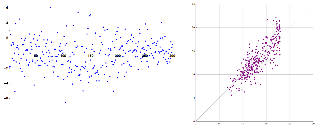
ListPlot[(data1 - data2), LabelStyle -> {14, GrayLevel[0], Bold},
PlotStyle -> Blue, ImageSize -> 700, PlotRange -> All]
pairs = Transpose[{data1, data2}];
ListPlot[pairs, Mesh -> All, ImageSize -> 500, AspectRatio -> Automatic,
PlotRange -> {{0, 25}, {0, 25}}, TicksStyle -> Directive[Black, 10],
AxesStyle -> Directive[Black, 12], Ticks -> Automatic,
GridLines -> Automatic, Axes -> True, PlotStyle -> {PointSize[.01], Purple},
Epilog -> Line[{{0, 0}, {25, 25}}]]
 Attachments:


