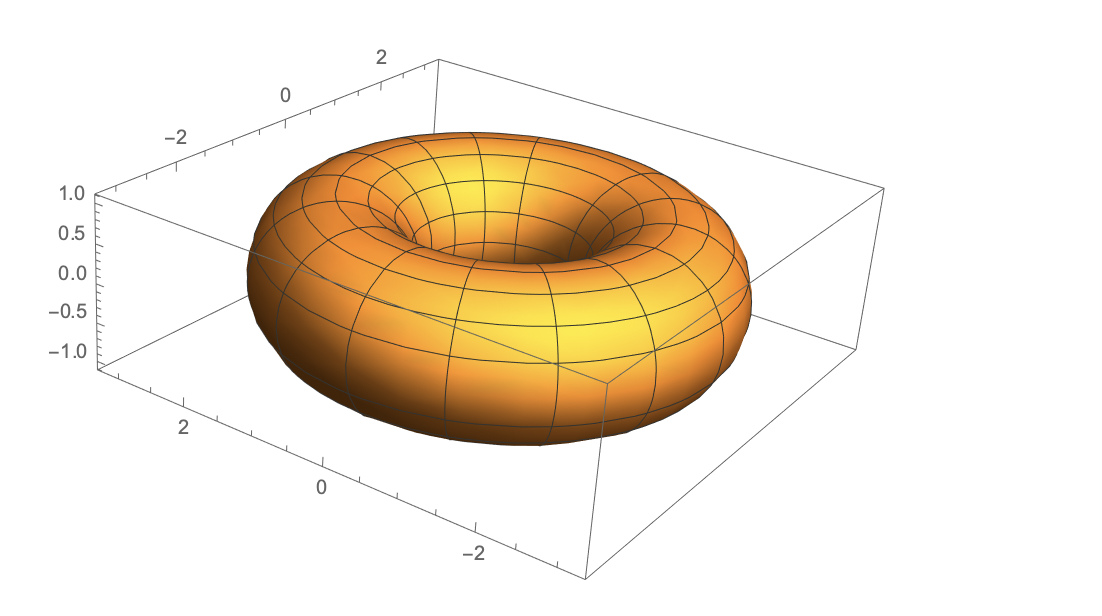
In this post, I will share the code and methods I used to solve the wave equation on a torus. To construct a solution to the wave equation on a torus, we need the Laplace-Beltrami operator from differential geometry. For more information on this operator, I recommend looking at this paper: http://www.math.mcgill.ca/toth/spectral%20geometry.pdf. Define coordinates, dimension, surface, and metric:
n = 2; coords = {u, v};
surf = {Cos[u] (2 + Cos[v]), (2 + Cos[v]) Sin[u], Sin[v]};
g =
FullSimplify[
Table[D[surf, coords[[i]]].D[surf, coords[[j]]], {i, 1, n}, {j, 1,
n}]];
ParametricPlot3D[surf, {u, 0, 2 \[Pi]}, {v, 0, 2 \[Pi]}]
Find the inverse metric:
ginv = Inverse[g];
Find the determinant of the metric:
detg = Det[g];
For some extra fun, we can find the Christoffel symbols of the second kind, the Riemann curvature tensor, the Ricci curvature tensor, and the Riemann scalar curvature:
\[CapitalGamma] =
  FullSimplify[ginv.Table[
     1/2 (D[g, coords[[j]]][[k, i]] +
        D[g, coords[[i]]][[k, j]] -
        D[g, coords[[k]]][[i, j]]), {k, 1, n}, {i, 1, n}, {j,
       1, n}]];
riemann =
  FullSimplify[
   Table[Sum[
     D[\[CapitalGamma][[l, i, k]], coords[[j]]] -
      D[\[CapitalGamma][[l, i, j]],
       coords[[k]]] + \[CapitalGamma][[l, j, s]] \[CapitalGamma][[s,
        i, k]] - \[CapitalGamma][[l, k, s]] \[CapitalGamma][[s, i,
        j]], {s, 1, n}], {l, 1, n}, {i, 1, n}, {j, 1, n}, {k, 1, n}]];
ricci = FullSimplify[
   Sum[Table[
     D[\[CapitalGamma][[l, i, j]], coords[[l]]] -
      D[\[CapitalGamma][[l, i, l]],
       coords[[j]]] + \[CapitalGamma][[m, i, j]] \[CapitalGamma][[l,
        l, m]] - \[CapitalGamma][[m, i, l]] \[CapitalGamma][[l, j,
        m]], {i, 1, n}, {j, 1, n}], {m, 1, n}, {l, 1, n}]];
scalar = FullSimplify[
   Sum[ginv[[i, j]] ricci[[i, j]], {i, 1, n}, {j, 1, n}]];
However, what really interests us is the Laplace-Beltrami operator.
\[ScriptCapitalL][f_, coord_] :=
  Sum[1/Sqrt[
      det[g] D[ginv[[\[Mu], \[Nu]]] Sqrt[
       detg] D[f, coord[[\[Nu]]]], coord[[\[Mu]]]], {\[Mu],
    1 n}, {\[Nu], 1, n}];
To solve a differential equation on a torus, we first need to create a gluing diagram to represent how our coordinates u and v map on to the torus:
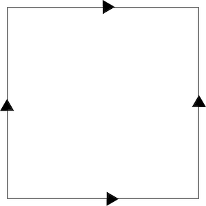
We can define our quotient space:
quotientspace = Rectangle[{0, 0}, {2 \[Pi], 2 \[Pi]}];
We then need to specify appropriate boundary conditions. I will use the PeriodicBoundaryConditions symbol allowing us to connect the two edges of the gluing diagram. This can also be thought of as creating a large grid of squares where the solution to the partial differential equation repeats itself in each square.
bcs = {PeriodicBoundaryCondition[\[Psi][t, u, v], u == 2 \[Pi],
   TranslationTransform[{-2 \[Pi], 0}]],
  PeriodicBoundaryCondition[\[Psi][t, u, v], v == 2 \[Pi],
   TranslationTransform[{0, -2 \[Pi]}]];
We then should specify some options:
opts = Method -> {"MethodOfLines", "TemporalVariable" -> t,
    "SpatialDiscretization" -> {"FiniteElement",
      "MeshOptions" -> {"MaxCellMeasure" -> 0.001}}};
Let's solve with the initial conditions being a small bump at u = Pi and v = Pi.
sol = NDSolveValue[{\[ScriptCapitalL][ \[Psi][t, u, v], coords] -
      D[\[Psi][t, u, v], {t, 2}] == 0,
    bcs, \[Psi][0, u, v] ==
     Exp[-(8 (u - \[Pi]))^2 - (8 (v - \[Pi]))^2],
    Derivative[1, 0, 0][\[Psi]][0, u, v] == 0}, \[Psi], {t, 0,
    10}, {u, v} \[Element] quotientspace, opts];
To visualize the solution, we will use a color function. Let's define the color function first.
colorf=Function[t, Function[{x,y,z,u,v},ColorData["FuchsiaTones"][Rescale[sol[t,u,v],{-.1/3,.1/3}]]]];
To animate, we need to generate a set of frames:
frames = ParallelTable[
   ParametricPlot3D[surf, {u, 0, 2 \[Pi]}, {v, 0, 2 \[Pi]},
    MeshFunctions -> Automatic, ColorFunction -> colorf[t],
    ColorFunctionScaling -> False, Boxed -> False, Axes -> False,
    ViewPoint -> {0, 15, 10}], {t, 0, 10, 1/30}];
Putting this all together in combination with some heavy computing power (thanks Boston University SCC), we get an animation that can be found at this link: https://drive.google.com/file/d/1gf0fMxZeMSInLbLemtFkvg1cGDb5ss/view?usp=sharing. Here are some screenshots from that animation: 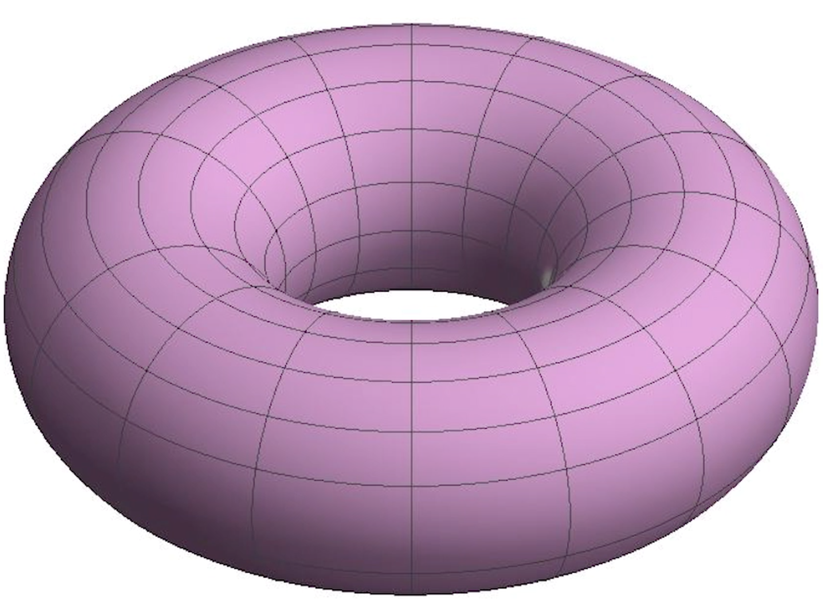
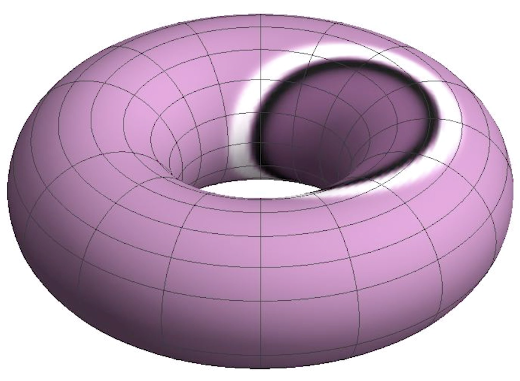
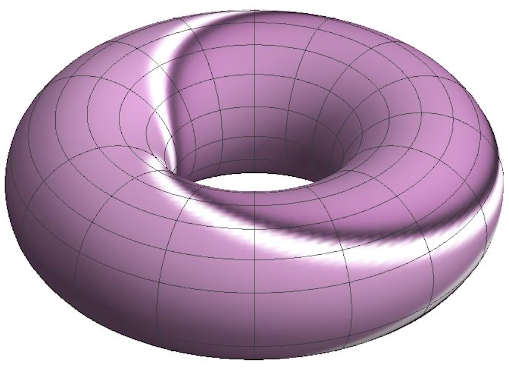
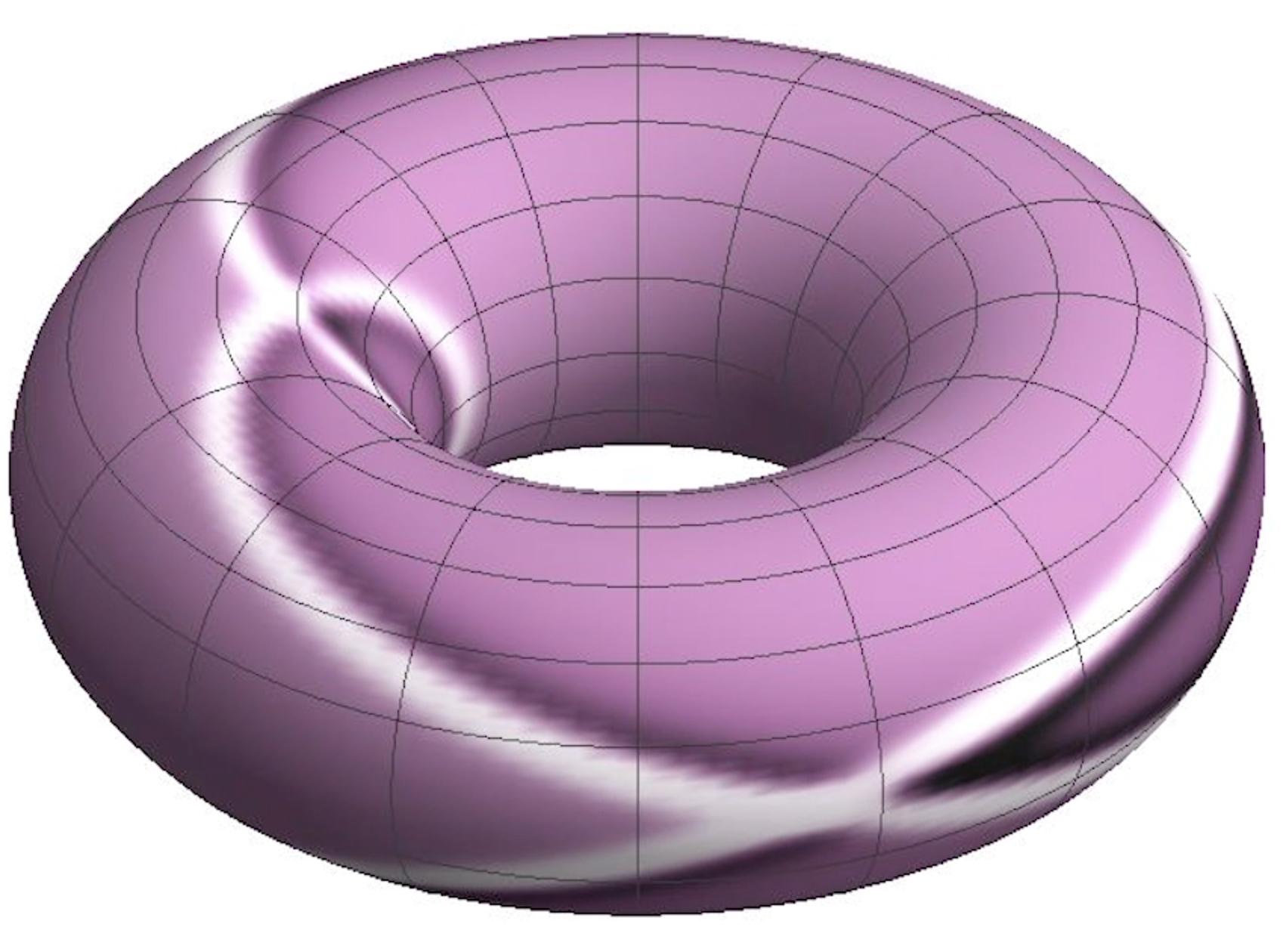
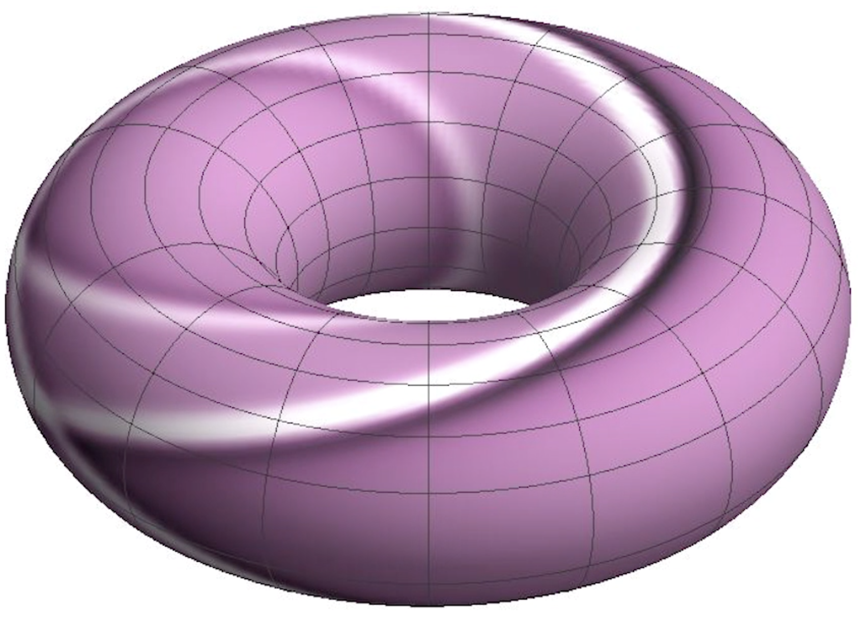
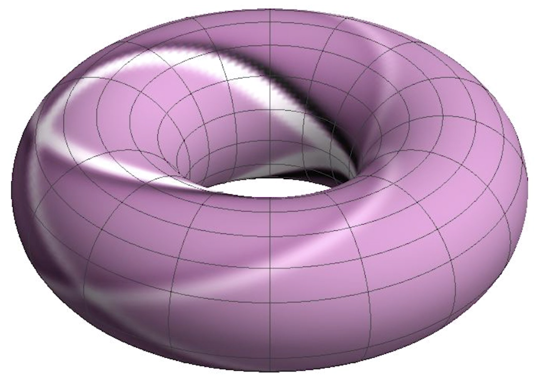
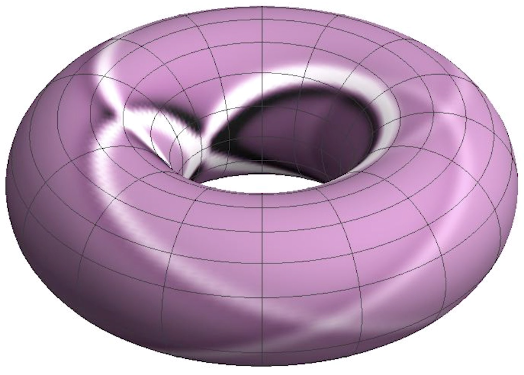
As seen in the animation the PeriodicBoundaryCondition allows the wave to interact with itself. The interaction of the wave with itself creates an increasingly chaotic solution. From my experience adjusting the size of the torus and the size of the initial bump. There is one additional representation I would like to leave you with. We can represent the solution by multiplying the solution by the tangent vector to create a torus that 'wiggles.'
frames = Table[
   ParametricPlot3D[{Cos[
       u] (2 + (1 + 1.2 \[Psi][t, u, v]) Cos[
          v]), (2 + (1 + 1.2 \[Psi][t, u, v]) Cos[v]) Sin[u],
     Sin[v]}, {u, 0, 2 \[Pi]}, {v, 0, 2 \[Pi]},
    ViewPoint -> {0, 15, 10}, PlotRange -> 3.5, Boxed -> False,
    Axes -> False], {t, 0, 20, .1}];
 Attachments:


