Hi All,
I just published a blog post proclaiming the implementation of a Mathematica package for quantile regression through linear programming. The blog post has couple of examples and several reference links:
http://mathematicaforprediction.wordpress.com/2013/12/16/quantile-regression-through-linear-programming/The implementation with Minimize is fairly straightforward. The linear programming implementation is slightly harder and also care has to be taken when the data has negative values.
Mathematica code difnitions:
QuantileRegressionFit::"nmat" = "The first argument is expected to be a matrix of numbers with two [/size][size=2]columns.";
QuantileRegressionFit::"fvlen" = "The second argument is expected to be list of functions to be fitted with at least one element.";
QuantileRegressionFit::"nvar" = "The third argument is expected to be a symbol.";
QuantileRegressionFit::"nqntls" = "The fourth argument is expected to be a list of numbers representing quantiles.";
QuantileRegressionFit::"nmeth" = "The value of the method option is expected to be LinearProgramming, Minimize, or a list with LinearProgramming or Minimize as a first element.";
QuantileRegressionFit::"mmslow" = "With the method Minimize the computations can be very slow for large data sets.";
Clear[QuantileRegressionFit]
Options[QuantileRegressionFit] = {Method -> LinearProgramming};
QuantileRegressionFit[data_, funcs_, var_, qsArg_, opts : OptionsPattern[]] :=
Block[{mOptVal, qs},
qs = If[NumericQ[qsArg], {qsArg}, qsArg];
(*This check should not be applied because the first function can be a constant.*)
(*!Apply[And,Map[!FreeQ[#,var]&,funcs]],Message[
LPQuantileRegressionFit::\"fvfree\"],*)
Which[
! (MatrixQ[data] && Dimensions[data][[2]] >= 2),
Message[LPQuantileRegressionFit::"nmat"]; Return[{}],
Length[funcs] < 1,
Message[LPQuantileRegressionFit::"fvlen"]; Return[{}],
Head[var] =!= Symbol,
Message[LPQuantileRegressionFit::"nvar"]; Return[{}],
! VectorQ[qs, NumericQ[#] && 0 <= # <= 1 &],
Message[LPQuantileRegressionFit::"nqntls"]; Return[{}]
];
mOptVal = OptionValue[QuantileRegressionFit, Method];
Which[
mOptVal === LinearProgramming,
LPQuantileRegressionFit[data, funcs, var, qs],
ListQ[mOptVal] && mOptVal[[1]] === LinearProgramming,
LPQuantileRegressionFit[data, funcs, var, qs, Rest[mOptVal]],
mOptVal === Minimize,
MinimizeQuantileRegressionFit[data, funcs, var, qs],
ListQ[mOptVal] && mOptVal[[1]] === Minimize,
MinimizeQuantileRegressionFit[data, funcs, var, qs, Rest[mOptVal]],
True,
Message[QuantileRegressionFit::"nmeth"]; Return[{}]
]
];
Clear[LPQuantileRegressionFit]
LPQuantileRegressionFit[dataArg_?MatrixQ, funcs_, var_Symbol, qs : {_?NumberQ ..}, opts : OptionsPattern[]] :=
Block[{data = dataArg, yMedian = 0, yFactor = 1, yShift = 0, mat, n = Dimensions[dataArg][[1]], pfuncs, c, t, qrSolutions},
If[Min[data[[All, 2]]] < 0,
yMedian = Median[data[[All, 2]]];
yFactor = InterquartileRange[data[[All, 2]]];
data[[All, 2]] = Standardize[data[[All, 2]], Median, InterquartileRange];
yShift = Abs[Min[data[[All, 2]]]];(*this is Min[
dataArg\[LeftDoubleBracket]All,2\[RightDoubleBracket]]-Median[
dataArg\[LeftDoubleBracket]All,2\[RightDoubleBracket]]*)
data[[All, 2]] = data[[All, 2]] + yShift ;
];
pfuncs = Map[Function[{fb}, With[{f = fb /. (var -> Slot[1])}, f &]], funcs];
mat = Map[Function[{f}, f /@ data[[All, 1]]], pfuncs];
mat = Map[Flatten, Transpose[Join[mat, {IdentityMatrix[n], -IdentityMatrix[n]}]]];
qrSolutions =
Table[
c = Join[ConstantArray[0, Length[funcs]], ConstantArray[1, n] q, ConstantArray[1, n] (1 - q)];
t = LinearProgramming[c, mat, Transpose[{data[[All, 2]], ConstantArray[0, n]}], opts];
If[! (VectorQ[t, NumberQ] && Length[t] > Length[funcs]), ConstantArray[0, Length[funcs]], t]
, {q, qs}];
If[yMedian == 0 && yFactor == 1,
Map[funcs.# &, qrSolutions[[All, 1 ;; Length[funcs]]]],
Map[Expand[yFactor ((funcs.#) - yShift) + yMedian] &, qrSolutions[[All, 1 ;; Length[funcs]]]]
]
];
Clear[MinimizeQuantileRegressionFit]
MinimizeQuantileRegressionFit[data_?MatrixQ, funcs_, var_Symbol, qs : {_?NumberQ ..}, opts : OptionsPattern[]] :=
Block[{minFunc, Tilted, QRModel, b, bvars, qrSolutions},
If[Length[data] > 300,
Message[QuantileRegressionFit::"mmslow"]
];
bvars = Array[b, Length[funcs]];
Tilted[t_?NumberQ, x_] := Piecewise[{{(t - 1) x, x < 0}, {t x, x >= 0}}] /; t <= 1;
QRModel[x_] := Evaluate[(bvars.funcs) /. var -> x];
qrSolutions =
Table[
minFunc = Total[(Tilted[q, #1[[2]] - QRModel[#1[[1]]]] &) /@ data];
Minimize[{minFunc}, bvars, opts]
, {q, qs}];
Map[funcs.# &, qrSolutions[[All, 2, All, 2]]]
];
Data generation function definition:
Clear[LogarithmicCurveWithNoise]
LogarithmicCurveWithNoise[nPoints_Integer, start_?NumberQ, end_?NumberQ] :=
Block[{data},
data =
Table[{t, 5 + Log[t] + RandomReal[SkewNormalDistribution[0, Log[t]/5, 12]]}, {t, Rescale[Range[1, nPoints],{1, nPoints}, {start, end}]}];
data
];
Data generation:
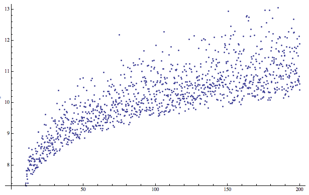
data = LogarithmicCurveWithNoise[1200, 10, 200];
ListPlot[data]
Regression quantiles calculation:
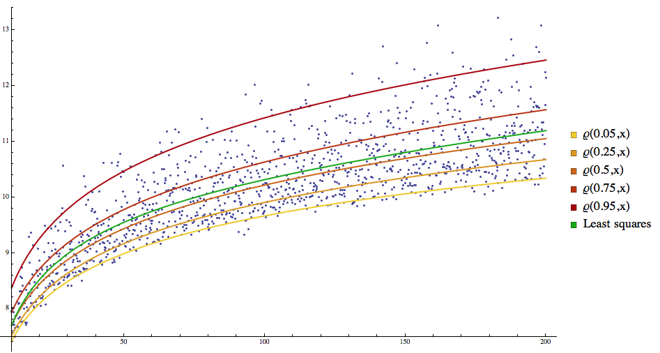
qs = {0.05, 0.25, 0.5, 0.75, 0.95};
qrFuncs = QuantileRegressionFit[data, {1, x, Sqrt[x], Log[x]}, x, qs]
"Standard" fit:
fFunc = Fit[data, {1, x, Sqrt[x], Log[x]}, x]
Plot all the curves together:
grData = ListPlot[data, PlotRange -> All];
grQReg = Plot[Evaluate[MapThread[Tooltip[#1, #2] &, {Append[qrFuncs, fFunc], Append[Map["\[CurlyRho](" <> ToString[#] <> ",x)" &, qs], "Least squares"]}]], {x, Min[data[[All, 1]]], Max[data[[All, 1]]]}, PlotStyle -> Append[Table[{AbsoluteThickness[2], Blend[{Yellow, Darker[Red]}, i/Length[qs]]}, {i, Length[qs]}], {AbsoluteThickness[2], Darker[Green]}], PlotLegends -> SwatchLegend[Append[Map["\[CurlyRho](" <> ToString[#] <> ",x)" &, qs], "Least squares"]]];
Show[{grData, grQReg}, ImageSize -> 600]