Open Code in Cloud
Introduction
The Wolfram Language Microcontroller Kit, which is part of the recently released version 12 of Mathematica, automates the generation and deployment of code to microcontrollers from the Wolfram Language. It supports several Adafruit development boards. So now you can take controllers, filters, or other systems models developed using the Wolfram Language and see them in action in the real world.
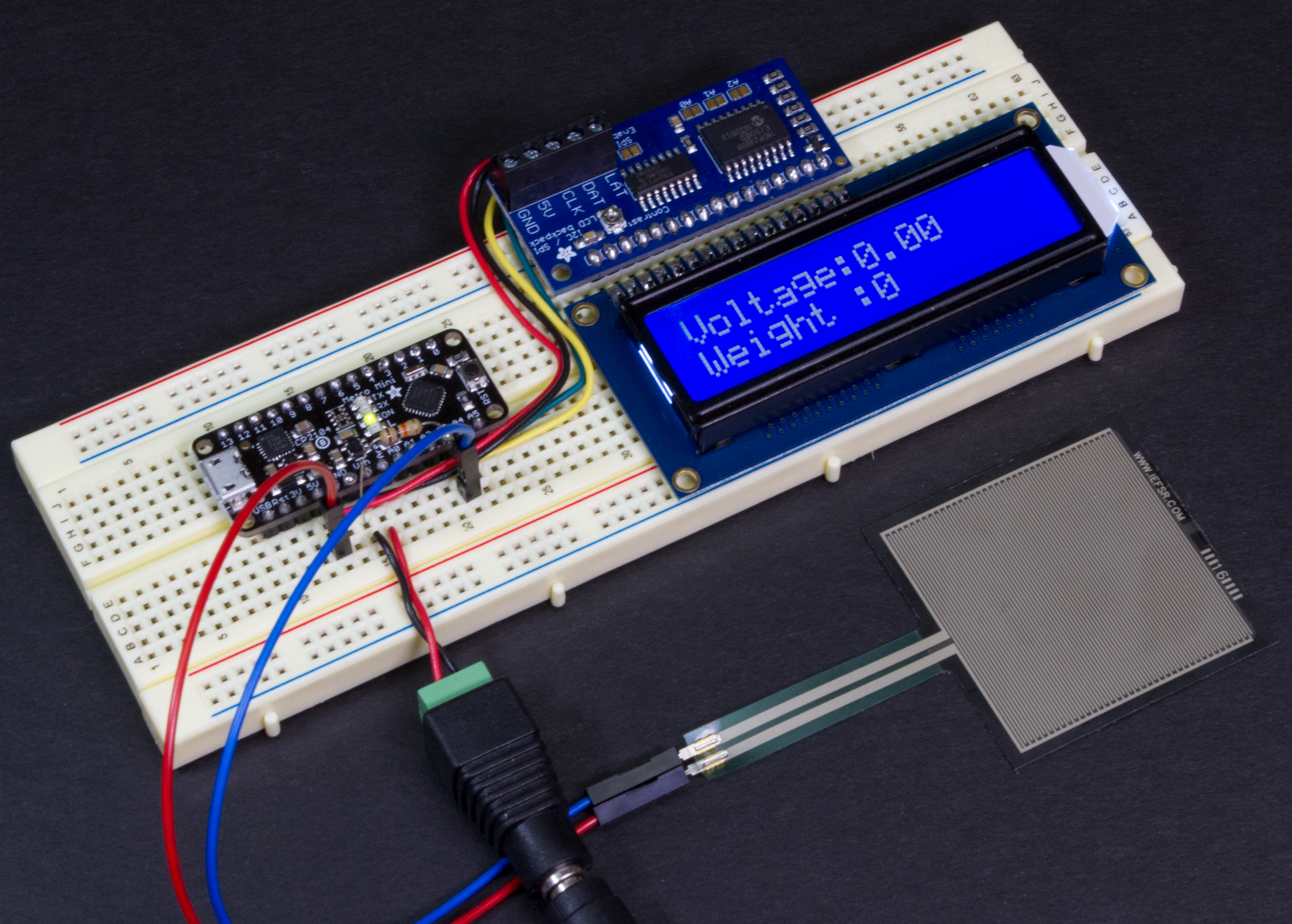
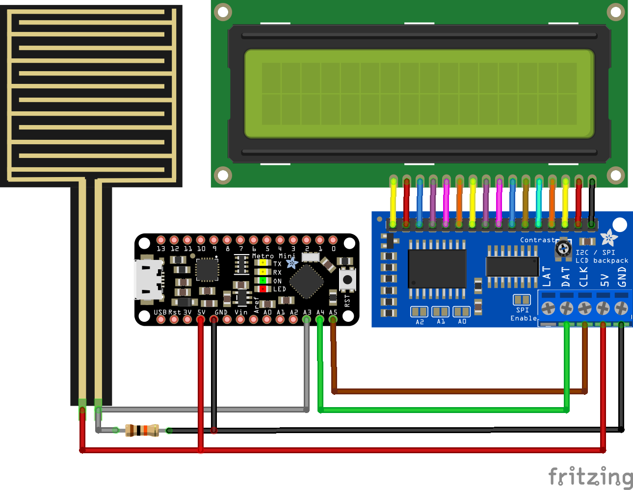
To showcase the Microcontroller Kit with an Adafruit development board, I will outline a basic analysis I did with a Force-sensitive Resistor (FSR). Since the functionality is designed with an unified interface, the workflow for another board, or input, or output channel follows essentially the same paradigm.
The following are the primary components I am using:
- Adafruit Metro Mini
- FSR
- 10 k[CapitalOmega] resistor
- LCD
- LCD backpack
The backpack is a nifty module because is drastically reduces the wiring and the number of microcontroller pins that need to be assigned to the LCD.
Obtain a model
The FSR is essentially a variable resistor whose resistance drops as the load on it increases. When there is no load the sensor theoretically has infinite resistance and acts at an open switch. If we connect one end of the sensor to a voltage Subscript[V, in] and the other end to ground through a pull-down resistor, the voltage v will be 0 when there is no load. Since this is a voltage divider configuration, the voltage v will increase as the load increases, and this analog signal will serve as a measure of the load on the sensor.
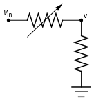
So I connected the FSR as shown in the above schematic, and measured the voltage v for various weights.
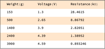
weights = {153, 500, 1400, 2400, 3900};
voltages = {1.3, 2.65, 3.9, 4.39, 4.59};
Then I computed the resistance values.
voltageDiv[v_, r_] := (v == 10/(10 + r) 5)
resistances = Table[r /. First[NSolve[voltageDiv[v, r], r]], {v, voltages}]
{28.4615, 8.86792, 2.82051, 1.38952, 0.893246}
This is a grid showing the weights used and the corresponding voltage and resistance values.
Grid[Join[{{"Weight(g)", "Voltage(V)",
    "Resistance(k\[CapitalOmega])"}},
  Thread[{weights, voltages, resistances}]], Alignment -> Left,
 Background -> {None, {{LightOrange, White}}}, Frame -> True,
 Spacings -> {4, 1.5}]
The log values of the resistance and weight have a linear relationship.
ListLogLogPlot[Thread[{resistances, weights}],
 PlotMarkers -> Automatic, Joined -> True, GridLines -> Automatic,
 Frame -> True,
 FrameLabel -> {"Resistance (k\[CapitalOmega])", "Weight (g)"}]
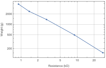
So I compute the mathematical relationship between the weight and the sensor's resistance, after first computing the linear relationship between their log values.
logValues = Map[Log, Thread[{resistances, weights}], {2}] // N
> {{3.34855, 5.03044}, {2.18244, 6.21461}, {1.03692, 7.24423}, {0.32896, 7.78322}, {-0.112893, 8.26873}}
LinearModelFit[logValues, r, r]
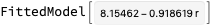
fitR = Power[E, %[Log[r]]]

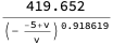
Then I express the resistance in terms of the voltage, to get the relationship between the weight and the measured voltage.
fit = fitR /. First[Solve[voltageDiv[v, r], r]]
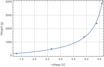
The derived relationship seems to be a good fit for the data.
p1 = Show[
  ListPlot[Thread[{voltages, weights}], PlotMarkers -> Automatic,
   GridLines -> Automatic, Frame -> True,
   FrameLabel -> {"voltage (V)", "Weight (g)"}],
  Plot[fit, {v, 0.01, 4.9}, PlotRange -> All]]
However, there are two problems with this model.
First, the expression's structure causes division by 0 at 0 V.
fit /. v -> 0
0.
Although the fitted weight should just be 0 .
Limit[fit, v -> 0]
0.
So I adjust the expression.
fit1 = fit /. Power[x_, p_ /; ! IntegerQ[p]] :> 1/Power[1/Together[x], p]
fit1 /. v -> 0
0.
And make sure I have adjusted it only structurally.
FullSimplify[fit1 - fit, 0 <= v < 5]
0.
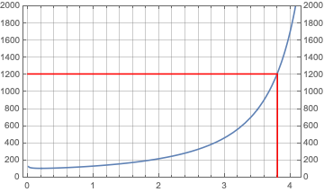
The second problem with the model is that the weight becomes unbounded as voltage approaches 5V.
Limit[fit, v -> 5]
Indeterminate
The sensor has a max load capability of 10,000 grams. So even voltage readings slightly below 5V are meaningless.
Grid[{{Plot[{fit, 10000}, {v, 4.5, 4.95}, PlotRange -> All,
    GridLines -> Automatic, Frame -> True,
    FrameLabel -> {"voltage (V)", "Weight (g)"}, Axes -> None,
    ImageSize -> 400,
    Filling -> {1 -> {{2}, {LightGreen, LightYellow}}}],
   Grid[Table[{v, fit}, {v, 4.7, 5.1, 0.05}], Alignment -> Left,
    Background -> {None, {{LightOrange, White}}}, Frame -> True,
    Spacings -> {2, 1}]}}, Spacings -> 3, Alignment -> Top]
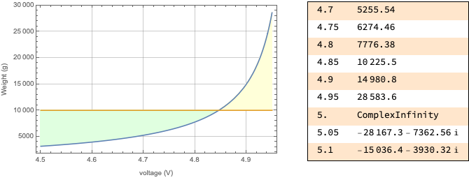
I compute the voltage reading would be for the upper limit of 9500 g.
maxV = v /. FindRoot[fit == 9500, {v, 4.99}]
4.83789
And create a systems model that will output -1 if the weight goes over the upper limit, and the fitted weight for readings below the limit.
sp = 1;
sys = NonlinearStateSpaceModel[{{}, { v,
    With[{maxV = maxV, fit = fit1},
     Which[ v > maxV, -1, True, fit]]}}, {}, {{v, 0}},
  SamplingPeriod -> sp]
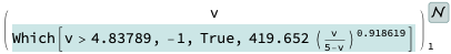
The model also outputs the measured voltage.
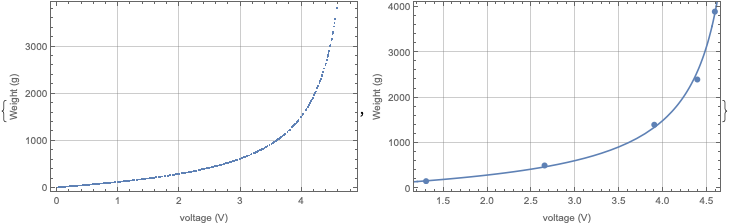
And as a quick sanity check, I plot the response of the systems model and make sure it agrees with the fitted model.
OutputResponse[sys, RandomReal[{0, maxV}, 500]];
Rasterize[#, ImageSize -> 350] & /@ {ListPlot[Transpose[%],
   GridLines -> Automatic, Frame -> True,
   FrameLabel -> {"voltage (V)", "Weight (g)"}, Axes -> None,
   ImageSize -> 350], Show[p1, ImageSize -> 350]}
Now, that I have the model, I can move on to setting up the microcontroller specifications.
Deploy the model
The FSR and the LCD backpack are connected to the microcontroller as shown below. The backpack needs to be wired or soldered to the LCD as described in the backpack tutorial.
Before I can deploy the model I also need to specify the input and output channels that connect to the model's input and outputs.
The input channel specification is simple. It's an analog signal from the sensor that is read on pin A3.
ic = "A3" -> "Analog";
To get the output to the LCD, I am using the Adafruit_LiquidCrystal library. For the Microcontroller Kit to use the library, I have to give the full path to the library.
lib = FileNameJoin[{$HomeDirectory, "Documents", "Arduino", "libraries", "Adafruit_LiquidCrystal"}];
DirectoryQ[lib]
True
I then go about integrating the library code into the generated code.
First, I list the files that need to be included.
incls = {"Wire.h", "Adafruit_LiquidCrystal.h"};
Next, I create an Adafruit_LiquidCrystal object. By default, the pads A0, A1, A2 on the backpack are not soldered which results in an I2C address 0.
util = "Adafruit_LiquidCrystal lcd(0)";
Next, I specify that it is a 16x2 LCD, set it up to turn on the backlight, and print the terms 'Voltage:' and 'Weight:' in the two rows.
inits = {"lcd.begin(16, 2)", "lcd.setBacklight(HIGH)", "lcd.setCursor(0, 0)",
"lcd.print(\"Voltage:\")", "lcd.setCursor(0, 1)", "lcd.print(\"Weight :\")"};
Then I get to the code that needs to run in the loop. The first output of the model sys is assigned to voltage and printed on the first row, while the second is assigned to weight and printed on the second row.
l1 = {"double voltage", "lcd.setCursor(8, 0)", "lcd.print(voltage)",
   "lcd.print(\"    \")"};

l2 = {"double weight", "lcd.setCursor(8, 1)", "lcd.print(round(weight))",
"lcd.print(\"    \")"};
Together they comprise the two output channels.
ocs = Table[<|"Type" -> "ExternalLibrary", "Loop" -> l|>, {l, {l1, l2}}];
And now I have the complete microcontroller specification.
?c = <|"Target" -> "AdafruitMetroMini328", "Inputs" -> ic,
"Outputs" -> ocs, "IncludeFiles" -> incls, "Utilities" -> util,
"Initializations" -> inits, "Timer" -> "delay"|>;
I connect the microcontroller to my laptop and determine the port that it is connected to. (The following works on both Mac and Linux. On Windows the port name is listed under COM ports in Device Manager.)
port = First[
FileNames[RegularExpression["cu\\..*(?i)(usb).+"],
FileNameJoin[{$RootDirectory, "dev"}]], "p"]
"/dev/cu.SLAB_USBtoUART"
And I upload the code to the microcontroller.
Needs["MicrocontrollerKit`"]

? = MicrocontrollerEmbedCode[sys, \[Mu]c, port, <|"Libraries" -> lib|>]
At this point, all the microcontroller needs is power and it will display a voltage and a weight reading on the LCD.
Observations and Conclusions
The FSR voltage reading tends to drifts upwards. Since the relationship with the measured weight looks like some kind of a probit function, a small variation in the voltage will result in a much larger variation in the weight reading. This can be monitored very clearly on an LCD where the voltage reading increases ever slightly causing much larger increases in the computed weight. The derivative of the fit will tell us the change in the weight. For example, at 3.8 V, a 0.01 V variation in voltage gives a (0.01 x 1200)12 gram variation in the weight.
With[{v1 = 3.8},
 With[{fit1 = fit /. v -> v1},
  Plot[Evaluate[D[fit, v]], {v, 0.01, 4.5},
   PlotRange -> {All, {0, 2000}}, Frame -> True,
   GridLines -> {Range[0, 4.5, 0.2], Range[0, 2000, 200]},
   FrameTicks -> {Automatic, Range[0, 2000, 200]},
   Epilog -> {Thickness[0.005], Red,
     Line[{{3.8, 0}, {v1, fit1}, {0, fit1}}]}]]]
Yet another issue with an FSR is inconsistency. The following are several samples of measured values and their fits.
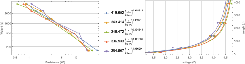
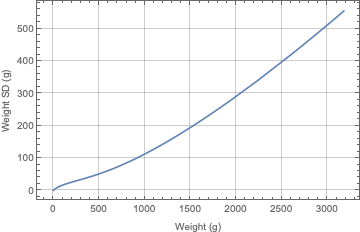
The standard deviation of the computed weights are higher at higher weights.
The data and the computations for the above plots can be found in this cloud notebook.
So while an FSR is not an accurate weighing sensor, it is useful for more qualitative things. Such as adjusting an analog output based on the weight...

Or turning on a digital output based on a threshold value...

As you can see, it is the same idiom that is repeated for various inputs and outputs, and also the targets and systems models. I have found this to be very useful when I want to test out a different target, or input or output configuration as it helps me to get the code deployed from a very high level specification and with very little effort.
Before closing, let me also mention that we haven't supported all the wonderful boards out there yet. The 1.0 release of the Microcontroller Kit supports the following Adafruit boards:


We will prioritize the boards for the next release for which there is strong interest. Please share suggestions in the comments below or email support@wolfram.com. If there are comments about this post or the Microcontroller Kit in general do post them as well.


