
Framing
An animated version of a graphic I produced for my paper "Stiefel manifolds and polygons", which appears in the Proceedings of Bridges 2019: Mathematics, Art, Music, Architecture, Education, Culture. The actual conference, which is an annual math art conference, happens in two weeks in Linz, Austria; if anybody is planning to attend, I will be giving a talk on Thursday, and also have two pieces (A to Z and Truncation) in the art exhibit.
To explain the animation a bit more: as I've mentioned before, there's a correpondence between polygons in space and points in the Grassmann manifold $G_2(\mathbb{C}^n)$ of 2-dimensional linear subspaces of $\mathbb{C}^n$ (by polygon in space I mean a closed, piecewise-linear curve in $\mathbb{R}^3$).
See that post for more details, but what I didn't mention there is that the correspondence is really between points in the Grassmannian and framed polygons, meaning that at each edge I have a triple of mutually perpendicular vectors: one pointing in the direction of the edge and the other two giving a perpendicular basis for the orthogonal complement of the edge direction (i.e., the normal space).
While we don't require these triples to be othonormal, we do require them to be mutually orthogonal and the same length, so we can think of the matrix whose columns are the vectors in the triple as a scaled element of $SO(3)$, the group of rotations of $\mathbb{R}^3$. Then the process of going from a framed polygon to the Grassmannian is the following: convert each scaled element of $SO(3)$ to a quaternion (formally, this means lifting to a scaled element of $\mathrm{Spin}(3)$), interpret the quaternion as $u + v j$, where $u$ and $v$ are complex numbers, let $\vec{u}$ and $\vec{v}$ be the complex $n$-vectors of the $u$'s and $v$'s, respectively, and then take the span of $\vec{u}$ and $\vec{v}$.
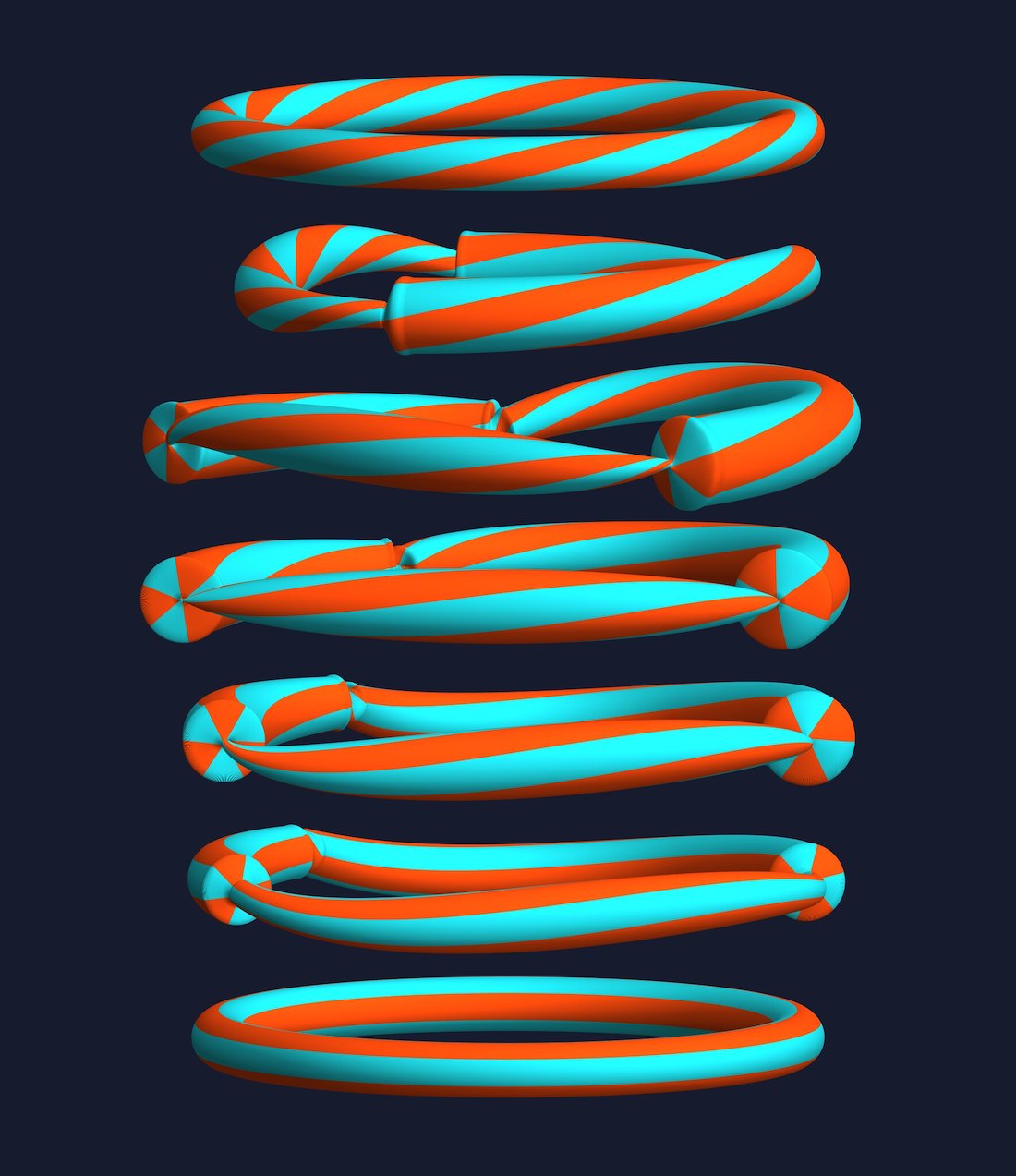
The virtue of doing this is that geodesics in the Grassmannian are easy to compute explicitly, which gives us a nice way of morphing between different framed polygons. The animation shows the geodesic in the Grassmannian between the $+3$-framed regular 200-gon (meaning that the frame vectors spin three times around the edge vectors as we travel all the way around the polygon), and the 0-framed 200-gon (in this case the frame vectors just always point straight up and straight out). The curves on the surface are all parallel to the paths traced out by the frame vectors.
It's probably not a coincidence that there are 3 singularities and we're going from a $+3$-framed polygon to a 0-framed polygon: getting rid of twist in the framing is expensive, and it seems to optimal to scale some edges down near length 0, then twist, then scale back up, so one needs to do this three times to get rid of three twists in the framing.
There's a fair amount of code that goes into this. First of all, we need to get the Quaternions package:
<< Quaternions`
Also, a couple of helper functions for converting between real and complex matrices:
Real4nToComplex2n[M_] :=
  Transpose[Complex @@ # & /@ # & /@ (Partition[#, 2] & /@ Transpose[M])];
Complex2nToReal4n[M_] := Transpose[Flatten /@ (ReIm /@ Transpose[M])];
For lifting from a scaled element of $SO(3)$ to a quaternion, I'm using a slight modification of the function rotm2q from Reichlin's quaternion package for Octave:
MatrixToQuaternion[A_] := Module[{M, T, l, s, w, x, y, z},
   l = Norm[A[[1]]];
   M = 1/l A;
   T = Tr[M];
   Which[T > 0,
    s = 1/(2 Sqrt[T + 1]);
    w = 1/(4 s);
    x = s (M[[2, 3]] - M[[3, 2]]);
    y = s (M[[3, 1]] - M[[1, 3]]);
    z = s (M[[1, 2]] - M[[2, 1]]);,
    M[[1, 1]] > M[[2, 2]] && M[[1, 1]] > M[[3, 3]],
    s = 2 Sqrt[1 + M[[1, 1]] - M[[2, 2]] - M[[3, 3]]];
    w = (M[[2, 3]] - M[[3, 2]])/s;
    x = s/4;
    y = (M[[1, 2]] + M[[2, 1]])/s;
    z = (M[[1, 3]] + M[[3, 1]])/s;,
    M[[2, 2]] > M[[3, 3]],
    s = 2 Sqrt[1 + M[[2, 2]] - M[[1, 1]] - M[[3, 3]]];
    w = (M[[3, 1]] - M[[1, 3]])/s;
    x = (M[[1, 2]] + M[[2, 1]])/s;
    y = s/4;
    z = (M[[2, 3]] + M[[3, 2]])/s;,
    True,
    s = 2 Sqrt[1 + M[[3, 3]] - M[[1, 1]] - M[[2, 2]]];
    w = (M[[1, 2]] - M[[2, 1]])/s;
    x = (M[[1, 3]] + M[[3, 1]])/s;
    y = (M[[2, 3]] + M[[3, 2]])/s;
    z = s/4;
    ];
   Sqrt[l] {w, x, y, z}
   ];
On the other hand, to go from a point in the Grassmannian (or Stiefel manifold) to a framed polygon, we use these functions:
QuaternionFramedEdges[
   StiefelForm_] := {Conjugate[#] ** Quaternion[0, 1, 0, 0] ** #,
     Conjugate[#] ** Quaternion[0, 0, 1, 0] ** #,
     Conjugate[#] **
      Quaternion[0, 0, 0, 1] ** #} & /@ (Quaternion @@ # & /@
     Transpose[StiefelForm]);
QFramedEdges[StiefelForm_] :=
  List @@ #[[2 ;;]] & /@ # & /@ QuaternionFramedEdges[StiefelForm];
Next, geodesics in the Grassmannian are computed very straightforwardly: suppose $P_1$ and $P_2$ are our two 2-dimensional linear subspaces in $\mathbb{C}^n$. Then the idea is to find the orthonormal bases for $P_1$ and $P_2$ which are as close to each other as possible, and then simply directly rotate one to the other. More precisely, we want to find unit vectors $a_i \in P_i$ so that $|\langle a_1, a_2\rangle |$ is maximal, then find unit $b_i \in a_i^\bot \cap P_i$ that maximize $|\langle b_1, b_2\rangle |$. Then $(a_i,b_i)$ is an orthonormal basis for $P_i$, and we realize the geodesic from $P_1$ to $P_2$ while directly rotating $a_1$ to $a_2$ and simultaneously rotating $b_1$ to $b_2$ (with speeds chosen so that both rotation finish at the same time). In turn, an easy way to find $a_1$ and $b_1$ is that they are the leading eigenvectors of the linear map which orthogonally projects from $P_1$ to $P_2$, and then back from $P_2$ to $P_1$.
So here's some code for computing geodesics:
ComplexProjectionBasis[{A_, B_}, {C_, D_}] :=
  Eigenvectors[
   Transpose[{A, B}].Conjugate[{A, B}].Transpose[{C, D}].Conjugate[{C, D}], 2];

ComplexGrassmannianGeodesic[{A_, B_}, {C_, D_}, t_] :=
  Module[{a, b, c, d, cPerp, dPerp, dist1, dist2},
   {a, b} = Orthogonalize[ComplexProjectionBasis[{C, D}, {A, B}]];
   {c, d} = Orthogonalize[ComplexProjectionBasis[{A, B}, {C, D}]];
   {cPerp, dPerp} = {Normalize[c - Re[Conjugate[c].a]*a],
     Normalize[d - Re[Conjugate[d].b]*b]};
   dist1 = ArcCos[Re[Conjugate[c].a]];
   dist2 = ArcCos[Re[Conjugate[d].b]];
   {Cos[t*dist1]*a + Sin[t*dist1]*cPerp,
    Cos[t*dist2]*b + Sin[t*dist2]*dPerp}
   ];
Finally, then, we just need to define our two framed 200-gons:
circleframe = With[{n = 200},
   1/10 Real4nToComplex2n[
     Transpose[
      MatrixToQuaternion /@ (Table[
           Transpose@
            Prepend[{{-#[[i, 2]], #[[i, 1]], 0}, {0, 0, 1}}, #[[i]]],
           {i, 1, n}]
          &[Append[#, 0] & /@ N[CirclePoints[n]]])]]
   ];
circleframe2 = With[{n = 200}, 1/10 Real4nToComplex2n[
     Transpose[
      MatrixToQuaternion /@ (Table[
           Transpose@
            Prepend[
             RotationMatrix[
               6 ? i/n].{{-#[[i, 2]], #[[i, 1]], 0}, {0, 0, 1}}, #[[i]]],
           {i, 1, n}]
          &[Append[#, 0] & /@ N[CirclePoints[n]]])]]
   ];
And put everything together:
DynamicModule[{frame, n, f, g, h,
  cols = RGBColor /@ {"#f6490d", "#1dced8", "#161c2e"}},
 Manipulate[
  frame =
   Transpose[
    QFramedEdges[
     Complex2nToReal4n[
      ComplexGrassmannianGeodesic[circleframe, circleframe2, t]]]];
  f = Interpolation[
      Transpose[{N@Range[0, 1, 1/(Length[#] - 1)], #}]] &[
    Prepend[#, #[[-1]]] &[# - ConstantArray[Mean[#], Length[#]] &[
      Accumulate[frame[[1]]]]]];
  g = Interpolation[
      Transpose[{N@Range[0, 1, 1/(Length[#] - 1)], #}]] &[
    Prepend[#, #[[-1]]] &[frame[[2]]]];
  h = Interpolation[
      Transpose[{N@Range[0, 1, 1/(Length[#] - 1)], #}]] &[
    Prepend[#, #[[-1]]] &[frame[[3]]]];
  n = Length[frame[[1]]];
  ParametricPlot3D[
   f[t] + 3 (Cos[?] g[t] + Sin[?] h[t]), {t, 0, 1}, {?, 0, 2 ?},
   MeshFunctions -> {#5 &}, Mesh -> 5,
   MeshShading -> {cols[[1]], cols[[2]]}, MeshStyle -> None,
   PlotPoints -> 50, Boxed -> False,
   ViewPoint -> -100 Normalize[Cross[f[0.], f[.25]]],
   ViewVertical -> f[0.], ViewAngle -> ?/300, PlotRange -> 1/2,
   ImageSize -> {540, 540}, Axes -> False, Lighting -> "Neutral",
   Background -> cols[[-1]]],
  {t, 0., 1}]
 ]


