Education: Wolfram Language for Electronics
Introduction
The objective of this lesson is to provide students with tools for self-teaching. The subject of choice is Electronics, a field where it's easy to get lost in the practical applications of diverse techniques and not focus on the theoretical aspects that enable said applications.
The lesson is designed to follow a particular format:
- Theoretical explanations
- Short paragraphs, hierarchization of information in bullet-points
- Interactive graphs
- Simulations
- Interactive graphs + simulation of real-world applications
- Demonstrations
- Plug in your Arduino and see the results for yourself
Sample Section of Theory
We'll begin the lesson by plotting a square wave:
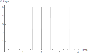
This square wave shows an alternation between 0 and 5 volts: We see 5 volts for a duration of half a second, then 0 volts for a duration of half a second.
- This wave can be read as "a square wave of 1Hz with a 50% duty cycle".
- Hz (Hertz) is the frequency of the wave. 1Hz means 1 cycle per second.
- Duty cycle is the portion of time during each cycle where the wave is at 5 volts, also known as "On" time (or HIGH in Arduino). 50% means that we have 5 volts for half the time and 0 volts for half the time.
If we were to connect an LED to a microcontroller pin outputting this wave, we'd get a blinking LED. In Arduino, we could do it with:
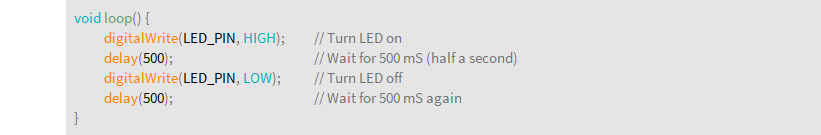
This will produce the following result:
Sample Section of Simulations
Now that we've seen what altering the frequency does, let's examine what happens when we alter the duty cycle between 10% and 100% at a constant frequency.
Sample Section of Demonstrations
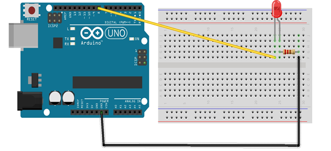
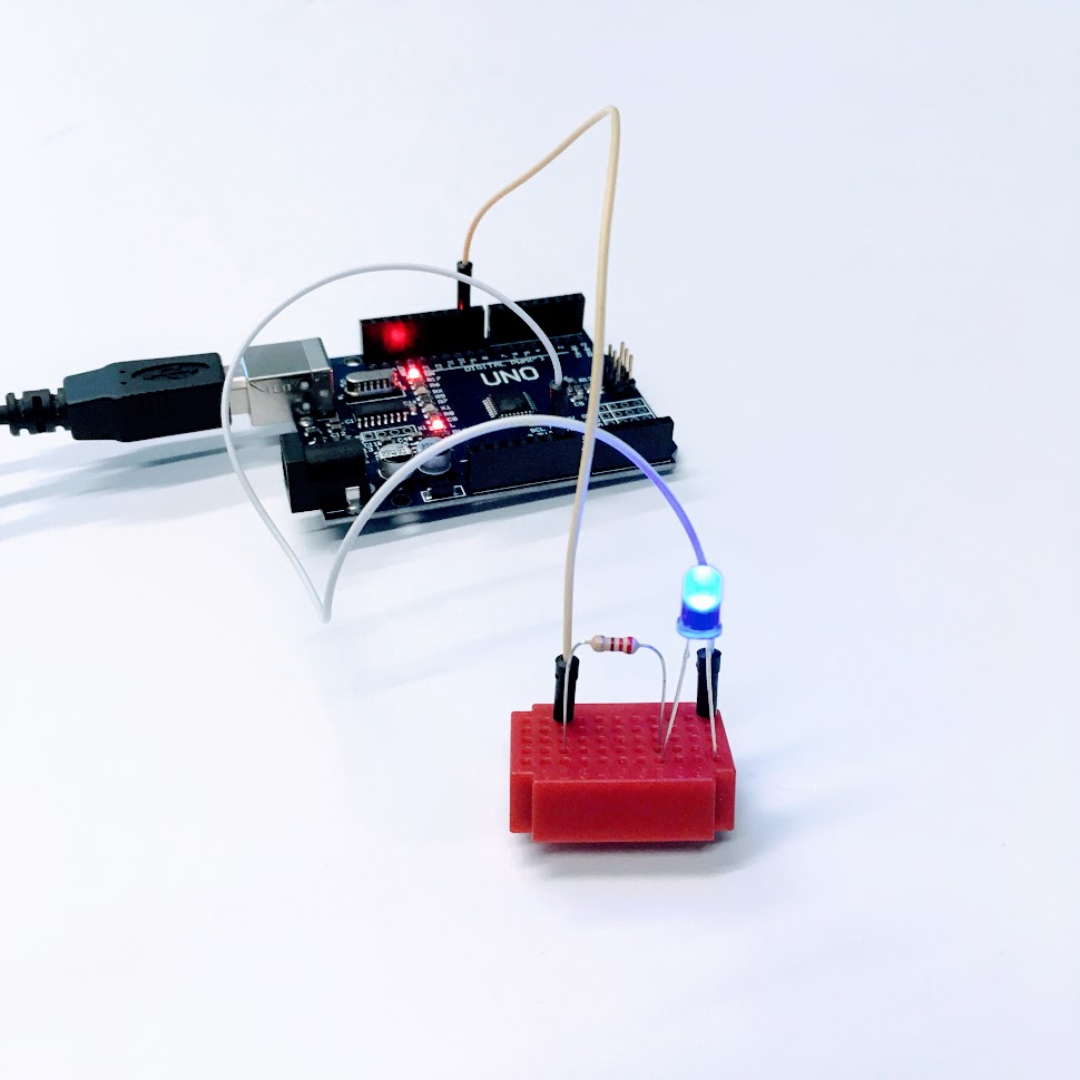
In order to demonstrate the concepts explained above, we are going to use Arduino. Connect an LED to pin 9 in series with a 220 Ohm resistor:
Next, let's do some setup. Enter the port where your Arduino is connected, here:
arduinoPort = "COM27";
Next, evaluate the following expression to connect to your Arduino:
arduino = DeviceOpen["Arduino", arduinoPort]

Let's start with the Frequency example. Input your desired frequency (in Hz) at the freq variable, then evaluate the expression.
Module[
 {freq = 5},
 Animate[
  Column[
   {ledSymbolF[onOff], DeviceWrite[arduino, 9 -> onOff]}], {onOff, 0,
   1, 1},
  DefaultDuration -> 1/freq,
  ContinuousAction -> True, AppearanceElements -> None,
  AnimationRunning -> False
  ]
 ]
Conclusions
The Wolfram Language is a powerful tool for lesson building, especially for self-teaching. The possibility to have interactive and animated graphs enables for more complex explanations in comprehensive ways. For electronics, the ability to manipulate directly a GPIO, and Arduino or a UART port makes real-world examples easy, in a single notebook.
Future Work
A full lesson plan embedded in a Raspberry Pi is the main objective. Add a touchscreen and a case, and the student will be equipped with a powerful self-teaching tool.
Behind the Scenes
Embedding circuit diagrams in a notebook is easy if you export them to PDF files -> a simple drag & drop to the notebook and Mathematica will process it into its native code. But if you want to animate a part of your diagram for interactive demonstrations or simulations, it can become tricky.
The way I'm doing this is by getting the InputForm of the embedded PDF:
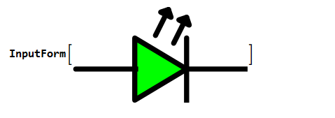
Evaluating that expression will return the parsed PDF file in Wolfram Language:
Graphics[{Thickness[0.005230818141333077], EdgeForm[{Thickness[0.029709200563967992], CapForm["Round"], JoinForm["Round"]}],
  FaceForm[{RGBColor[0., 1., 0.], Opacity[1.]}], FilledCurve[{{{0, 2, 0}}, {{0, 2, 0}, {0, 1, 0}, {0, 1, 0}, {0, 1, 0}}, {{0, 2, 0}}, {{0, 2, 0}},
    {{0, 2, 0}, {0, 1, 0}}, {{0, 2, 0}}, {{0, 2, 0}, {0, 1, 0}}}, {{{2.8789999999999996, 36.959115999999995}, {67.473, 36.959115999999995}},
    {{188.29299999999998, 36.959115999999995}, {124.27, 36.959115999999995}, {67.473, 71.037116}, {67.473, 2.880116000000001}, {124.27,
    36.959115999999995}}, {{124.27, 71.037116}, {124.27, 2.880116000000001}}, {{124.27, 93.755116}, {110.07, 65.35711599999999}}, {{115.75,
    90.916116}, {124.27, 93.755116}, {127.109, 85.236116}}, {{104.391, 102.275116}, {90.191, 73.877116}}, {{95.871, 99.435116}, {104.391,
    102.275116}, {107.23, 93.755116}}}]}, AspectRatio -> Automatic, ImageSize -> {192., 106.},
 PlotRange -> {{0., 191.17468299999996}, {0., 105.150116}}]
My specific goal was to dynamically change the color of the LED symbol for the simulations, so what I had to do was find the green color:
(...) FaceForm[{RGBColor[0., 1., 0.] (...)
We can see the the RGBColor[] function right at the top.
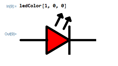
Finally, all I needed to do was put the whole input form into a function:
ledColor[r_, g_, b_] :=
 Graphics[{Thickness[0.005230818141333077],
   EdgeForm[{Thickness[0.029709200563967992], CapForm["Round"],
     JoinForm["Round"]}], FaceForm[{RGBColor[r, g, b], Opacity[1.]}],
   FilledCurve[{{{0, 2, 0}}, {{0, 2, 0}, {0, 1, 0}, {0, 1, 0}, {0, 1,
       0}}, {{0, 2, 0}}, {{0, 2, 0}}, {{0, 2, 0}, {0, 1, 0}}, {{0, 2,
       0}}, {{0, 2, 0}, {0, 1, 0}}}, {{{2.8789999999999996,
       36.959115999999995}, {67.473,
       36.959115999999995}}, {{188.29299999999998,
       36.959115999999995}, {124.27, 36.959115999999995}, {67.473,
       71.037116}, {67.473, 2.880116000000001}, {124.27,
       36.959115999999995}}, {{124.27, 71.037116}, {124.27,
       2.880116000000001}}, {{124.27, 93.755116}, {110.07,
       65.35711599999999}}, {{115.75, 90.916116}, {124.27,
       93.755116}, {127.109, 85.236116}}, {{104.391,
       102.275116}, {90.191, 73.877116}}, {{95.871,
       99.435116}, {104.391, 102.275116}, {107.23, 93.755116}}}]},
  AspectRatio -> Automatic, ImageSize -> {192., 106.},
  PlotRange -> {{0., 191.17468299999996}, {0., 105.150116}}]
Done! Now, calling the function will return the object with the parameters you specified:
Important Note: Try to avoid having text in your PDFs since it makes the input form extremely long. If you need to add text to your objects, a handy trick is to add tiny rectangles with specific colors in your PDF, in the position where the text would be. This way, you can find these markers and replace them with a variable where your strings will be.
Hope you find this trick useful and (remember that I'm a beginner Wolfram Language speaker) if there's a better, cleaner way to do this, I'd love to read about it!


