Introduction
The primary goal of this project was to create a function that uses vertex points of a given lattice to create tessellations of the plane. These tessellations could then be used to study cellular automata with cell shapes different from the usual squares. We chose to focus on 2 dimensional lattices, due to the ease with which they can be visualized, and used the (potentially skewed) regular tilings they induce for the cells of our cellular automata.
Lattices
Sparse Arrays as Lattices
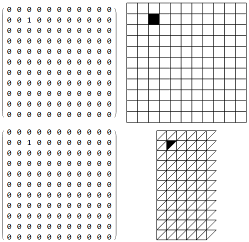
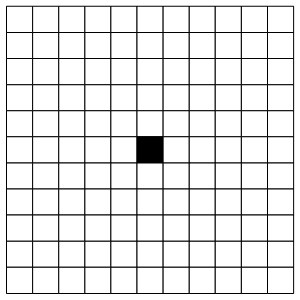
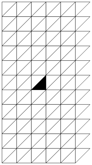
In a regular tessellation of a finite rectangular subset of $\mathbb{R}^2$ we can assign a pair of integers to each cell to represent it's coordinates. If one is careful and consistent about how they count, the same can be done with triangular and hexagonal tessellations. This, combined with the fact that we will also want to assign a value to each cell for CA representation purposes, means sparse arrays are a natural choice for representing and manipulating lattice cells. Naturally, a value of 0 corresponds to an empty (off) cell and a value of 1 corresponds to a filled-in (on) cell.
Grid[
{{SparseArray[{2, 3} -> 1, {11, 11}] // MatrixForm,
   LatticePlot[SparseArray[{2, 3} -> 1, {11, 11}], ImageSize -> 200]},
  {SparseArray[{2, 3} -> 1, {11, 11}] // MatrixForm,
   LatticePlot[SparseArray[{2, 3} -> 1, {11, 11}],
    "CellShape" -> Triangle, ImageSize -> 100]}}
]
Lattice Plotting
Plotting only the lattice points is fairly simple and can be done using the following code:
basis = {{1, 0}, {-0.5, Sqrt[3]/2}};
ListPlot[
    Flatten[
        Table[(i*basis[[1]] + j*basis[[2]]), {i, -5, 5}, {j, -5, 5}],
    1
    ]
]
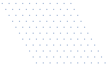
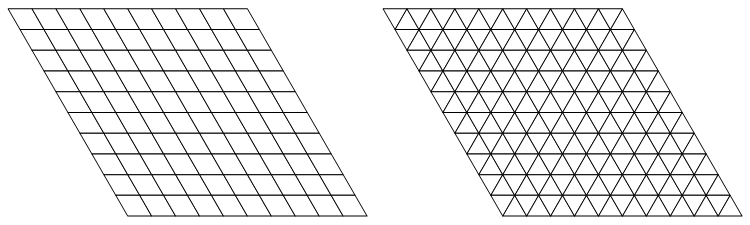
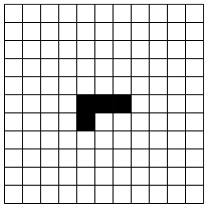
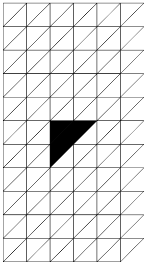
With the standard square tessellation filling in the edges is fairly straightforward, however when working with triangular or hexagonal arrays things get slightly more complicated as one has to account for the rotation and misalignment of neighboring cells. For now we decided to hard-code the way edges are plotted as this is simple in for 2 dimensional regular tilings, but in future work we would like to find a procedural way of solving this problem for more irregular 2 and 3 dimensional cell shapes. Below we include example tilings of the above lattice.
Cellular Automata
von Neumann Neighborhoods
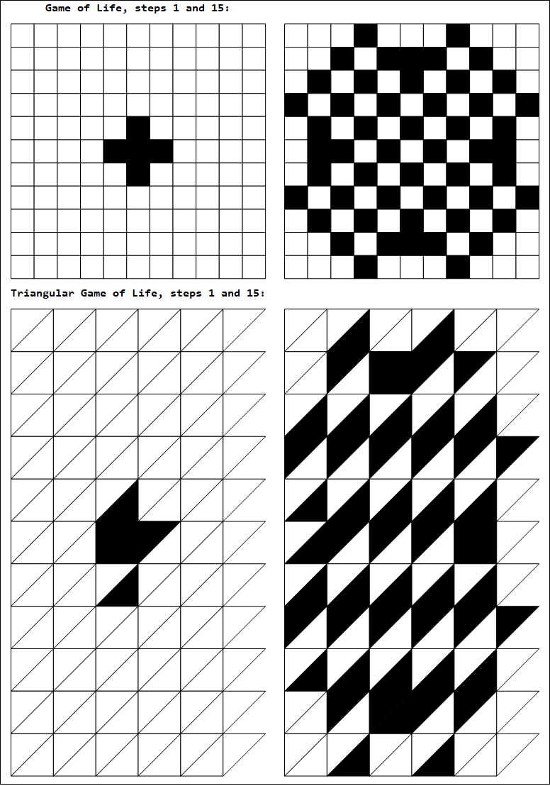
There are two kinds of neighborhoods commonly used to specify CA evolution rules: von Neumann Neighborhoods and Moore neighborhoods. We chose to focus on the first kind, as the definition of Moore neighborhoods doesn't readily translate to non-square cell cases. As before, finding the coordinates of the neighbors of a given cell is easy in the square (and cubic and hyper-cubic) cases, but gets much more difficult with more irregular shapes. We once again decided to hard-code the von Neumann neighborhoods of each given cell. This can be done as follows:
Options[vonNeumannNeighborhood]={"CellShape"->Square};

vonNeumannNeighborhood[cell_,lattice_,OptionsPattern[vonNeumannNeighborhood]]:=
Module[
    {c1=cell[[1]],c2=cell[[2]],s=OptionValue["CellShape"]},
    Which[
       s===Square,
         {c1,c2}->{{c1-1,c2},{c1,c2-1},{c1,c2},{c1,c2+1},{c1+1,c2}},

       s===Hexagon,
         If[OddQ[c1],
          {c1,c2}->{{c1-1,c2-1},{c1-1,c2},{c1,c2-1},{c1,c2},{c1,c2+1},{c1+1,c2-1},{c1+1,c2}},
          {c1,c2}->{{c1-1,c2},{c1-1,c2+1},{c1,c2-1},{c1,c2},{c1,c2-1},{c1+1,c2},{c1+1,c2+1}}
          ],
       s===Triangle,
         If[EvenQ[c2],
          {c1,c2}->{{c1,c2-1},{c1,c2},{c1,c2+1},{c1+1,c2-1}},
          {c1,c2}->{{c1-1,c2+1},{c1,c2-1},{c1,c2},{c1,c2+1}}
          ]
         ]
];
CA Rules
In general, any function $f:\mathbb{F}_2^n\times\mathbb{F}_n\rightarrow\mathbb{F}_2$, where $n$ is the order of the von Neumann neighborhood of a cell, can be used to specify a rule governing the evolution of a CA. Our code currently allows the user to specify rules of the form $f:\mathbb{F}_2\times\mathbb{F}_n\rightarrow\mathbb{F}_2$, where the first input is the current state of the cell and the second is the sum of the states of all cells in a von Neumann Neighborhood. Note that we set our boundary conditions to 0, but this can also be adjusted within the code.
Options[cellEvolution]:={"CellShape"->Square};

cellEvolution[cell_,globalState_,rule_,OptionsPattern[cellEvolution]]:=
Lookup[
    rule,{{cellState[cell,globalState],Total[neighborhoodState[cell,globalState]]}}][[1]];
Plotting and Animating CA
Once we have a method of displaying arrays as cells and manipulating those lattices as if they were a CA, actually displaying the CA is very easy. We simply apply the specified evolution rule to every cell and plot the resulting lattice using LatticePlot. The following code displays a CA after applying the evolution rule $n$ times to the initial state:
Options[CAPlot]:={"CellShape"->Square,ImageSize->300};

CAPlot[lattice_,func_Function,time_Integer:0,basis_List:{{1,0},{0,1}},OptionsPattern[CAPlot]]:=
Module[
    {vNN=vNNTable[lattice,"CellShape"->OptionValue["CellShape"]],timestate=Nest[globalEvolution[#,func,"CellShape"->OptionValue["CellShape"]]&,lattice,time]},
    Graphics[
       LatticePlot[
         timestate,
         basis,
         "CellShape"->OptionValue["CellShape"],
         ImageSize->OptionValue[ImageSize]
       ]
    ]
];
We can also animate CA's simply by storing the CA state after each application of the rule as a list and animating the result. The following code takes care of this for us:
Options[CAEvolution]:={"CellShape"->Square,ImageSize->300};

CAEvolution[lattice_,func_Function,time_Integer:10,basis_List:{{1,0},{0,1}},OptionsPattern[CAEvolution]]:=
Module[
    {vNN=vNNTable[lattice,"CellShape"->OptionValue["CellShape"]],timestate=NestList[globalEvolution[#,func,"CellShape"->OptionValue["CellShape"]]&,lattice,time]},
    Animate[
       LatticePlot[
         timestate[[n]],
         basis,
         "CellShape"->OptionValue["CellShape"],
         ImageSize->OptionValue[ImageSize]
       ],
    {{n,1},1,time,1},
    AnimationRate->2,
    AnimationRunning->False
    ]
];
and we can now generate pretty animations such as theses:
If you're interested, you can find our full code in the following GitHub repository.
References
- https://en.wikipedia.org/wiki/Cellular_automaton
- https://www.wolframscience.com/nks/


