Disclaimer
This computational notebook is not to be sold or exchanged for either monetary or non-monetary gains in anyway. The notebook is not to be modified without prior written consent from the author. ?The calculation only serves as an additional reference for equity investors and investment advisors. Any liability, including any liability for negligence, for any loss or damage arising from reliance on this computational notebook, is expressly excluded. Under no circumstance shall the author of this computational notebook or Wolfram Research be held responsible for third-party's application, investment recommendation, or other usage originating from this computational notebook.
I. Abstract
A quantitative model was derived to analyze common collections of investment tactics. The model was designed with flexibility: it can choose and weight the stocks into a portfolio of any size, based on any analytic expression of the stocks' financial characteristics, allowing both whole and fractional shares, with an option for additional investment. Using the model, several common investment strategies were investigated: chosen and weighted by price; chosen by price, equally weighted; chosen by volume, weighted by market capitalization; chosen and weighted by market capitalization. The model shows that a less frequently adjusted portfolio seems to perform better, supporting the buy-and-hold tactic. The model also indicate that the size of the portfolio, does not exert a strong effect on the strategy's overall performance.
II. Introduction
Equity investing remains a significant vehicle to preserve and generate wealth. Owing to the advances in technology and computational instruments, as well as the readily available financial data, strategical equity investing has become more technically accessible. Yet, apart from large financial institutions (such as hedge-funds and investment banks), the analyzing tools for investment strategies are not readily available to most individual investors - and even when the tools are available, the analysis are often basic and limited. Hence, a mathematically robust, versatile tool for investment strategy would enable more people to participate in investing, to make better-informed choice, which may narrows the standard of living gap between different social classes.
Here, a computational model was derived and freely distributed to help quantifying the most common collection of investment strategies: the model aims to quantify the portfolio's performance, in which stocks are chosen and weighted based on certain criteria. The model consists of two distinct parts: the gathering of historical data/financial information, and the construction of the portfolios - back-testing on historical data for theoretical performance (transactional fees and other necessary costs are not included in the model).
III. Data Gathering
ClearAll["Global`*"];
SetDirectory[NotebookDirectory[]];
First, a collection of stocks is specified: this collection will serve as the "set of all stocks", from which the portfolios will be constructed. For the purpose of constructing and testing a computational model, the collection is chosen to be SP500: all the stocks that are listed on the Standard and Poor 500 Index (^SPX)
listStock = EntityList[EntityClass["Financial", "SP500"]];
DumpSave["listStock.MX", listStock];
This specified "set of all stocks" SP500 is then associated with multiple other financial properties: price, option2, option3, option4, option5, option6. Price is always included, since stock price is necessary to quantify an investment strategy's performance. The other options are chosen from the following list, so that they result in timeseries (measurements over time) of the properties (as currently supported by Wolfram Mathematica kernel, 2019-07-10): {"Change", "Close", "CumulativeFractionalChange", "Dividend", "DividendPerShare", "Last", "MarketCap", "Open", "Price", "RawVolume", "Return", "Volume"}. If an option is not used, that option must be specified as "None".
The financial properties for the "set of all stocks" are collected with one call of FinanciaData[], in order to minimize the downloading time. Yet, because of the sheer size of the timeseries: all daily data points of several properties of all stocks since the stocks' inception, the financial properties may take as much as two hours to be procured (the Boolean variable run is used to prevent inadvertently overwriting the obtained data file - it needs to be changed to True in order to execute the codes in this section).
option2 = "MarketCap";
option3 = "Volume";
option4 = "Close";
option5 = "Open";
option6 = "None";
listOptions =
  DeleteCases[{option2, option3, option4, option5, option6}, "None"];
DumpSave["listOptions.MX", listOptions];

run = False;
If[run == True,
  listStockPropRaw =
   FinancialData[listStock, Prepend[listOptions, "Price"], All]];
The portfolios will be compared against a benchmark to assess their performance. This benchmark is chosen to be the Standard and Poor 500 Index (^SPX): the data is stored in sp500All variable.
sp500All = FinancialData["^SPX", All];
DumpSave["sp500All.MX", sp500All];
Once all the financial properties are (finally) obtained, the timeseries are changed into interpolation order of 0, which means missing/interval measurements will be identical to its immediately previous measurement, effectively describing a step function (instead of interpolating the interval measurement from both its immediate previous data point and its next data point - i.e. using future data to make a present decision). This step is crucial for back-testing, especially with quarterly (every three months) financial data such as dividend, total asset, total liability, EBITDA (earnings before interest, tax, depreciation and amortization), etc.
(At the moment, Wolfram Research has plan to incorporate EntityValue[] of entity "Company" into the FinancialData[] function, so that by querying a stock, the associated company's financial and accounting information can be obtained.)
If[run == True,
 listStockProp =
  Replace[listStockPropRaw,
   List["Interpolation", Rule[InterpolationOrder, 1]] ->
    List["Interpolation", Rule[InterpolationOrder, 0]], {5}];
 DumpSave["listStockProp.MX", listStockProp];
 ]
The SP500 stocks's name and financial properties are combined into one variable: masterThread, with its definition saved into "masterThreadGeneral.MX". The variable masterThread is ascertained with its length and an excerpt of its contents.
If[run == True,
 CompoundExpression[
  masterThreadNotIndexed =
   DeleteMissing[
    Transpose[Prepend[Transpose[listStockProp], listStock]],
    1, 3];

  masterThread =
   Transpose[
    Prepend[Transpose[masterThreadNotIndexed],
     Range[Length[masterThreadNotIndexed]]]];
  DumpSave["masterThreadGeneral.MX", masterThread];

  masterThread // Length
      RandomSample[masterThread, 5] // TableForm // Print
  ]]
For the sole purpose of constructing the computational model, a smaller set of 64 randomly selected stocks from SP500 are obtained (since making a portfolio by sorting the whole 505 stocks in the SP500 set would take a bit longer - which is unnecessary at this stage).
If[run == True,
 CompoundExpression[
  ClearAll[masterThread];
  masterThreadNotIndexedSample = RandomSample[
    DeleteMissing[
     Transpose[Prepend[Transpose[listStockProp], listStock]],
     1, 3], 64];

  masterThread =
   Transpose[
    Prepend[Transpose[masterThreadNotIndexedSample],
     Range[Length[masterThreadNotIndexedSample]]]];
  DumpSave["masterThreadSample64.MX", masterThread];

  masterThread // Length
     RandomSample[masterThread, 5] // TableForm // Print
  ]]
IV. Constructing the computational model
First, the previously constructed listOptions, sp500All, and the masterThread variables are reloaded into a clean Mathematica kernel.
ClearAll["Global`*"];
SetDirectory[NotebookDirectory[]];
Off[InterpolatingFunction::dmval];
Off[EntityValue::conopen];

Get["listOptions.MX"];
Get["sp500All.MX"];
Get["masterThreadGeneral.MX"];
The inputs for the computational model are specified:
timePeriod denotes the portfolio's frequency of adjustment in whole number of days: timePeriod = n means that the portfolio is updated/adjusted every n days.
sizePortfolio denotes the portfolio's size - the pre-specified number of stocks the portfolio contains. Obviously, the portfolio size must be smaller than the number of stocks in masterThread.
taxRate takes into account the rate of tax on capital gain. Here, the tax is set at 40% for any capital gain each time the portfolio is rebalanced, and immediately deducted. This setup is much more restrictive than the personal income tax schedule in the U.S.: rate depending on personal income (maximum 37%, 2019), calculated for the whole year, and not due until April of the following year.
initialInvest specifies the initial amount of money invested in the portfolio.
dailyInvest specifies the additional daily amount of money invested in the portfolio. Each time the portfolio is rebalanced, an amount of dailyInvest*timePeriod will be added into the portfolio.
optionWholeShare specified whether only whole numbers (positive integers) of stock share are allowed, or fractional shares are also possible, as some trading platforms permit whole share only. Variable optionWholeShare accepts only Boolean values True or False.
beginDate denotes the first date of the investigated time window.
endDate denotes the last date of the investigated time window.
funcSort[] determines how the stocks in masterThread (the "set of all stocks") at one specific instant of time are sorted for selection, from largest to smallest. Function funcSort accepts any analytic expression of x1, x2, x3, x4, x5,..., corresponding to the financial properties "Price", option2, option3, option4, option5,...
optionTake, which is linked to funcTake[] on the following paragraph, specified how the stocks are collected into a portfolio from the sorted masterThread (using funcSort). Variable optionTake is designed to accept only three designation: "high", meaning the largest stocks are taken (with respect to their metrics obtained from funcSort); "low", meaning the smallest stocks are taken; and mid", meaning the middle stocks are taken.
funcWeight[] determines how the selected stocks in the portfolio are weighted for investment. Function funcWeight accepts any analytic expression of x1, x2, x3, x4, x5,..., corresponding to the financial properties "Price", option2, option3, option4, option5,... To use funcWeight, optionEqualWeight must be False.
optionEqualWeight denotes whether to use funcWeight[], or to assign equal weight to all selected stocks in the portfolio. Variable optionEqualWeight accepts only Boolean values True or False.
Function funcTake[], mentioned earlier with variable optionTake, is defined to execute the input given to optionTake.
Variable sp500Ratio stores the relative value of the Standard and Poor 500 Index (^SPX) since the first date of the investigated time window - of which the portfolio performance is compared against.
timePeriod = 56;
sizePortfolio = 10;
taxRate = 0.4;
initialInvest = 100.00;
dailyInvest = 0.00;
optionWholeShare = False;

beginDate = DateObject["2004-07-01"];
endDate = DateObject["2019-07-01"];

funcSort[x1_, x2_, x3_, x4_, x5_] :=
  x2/10^6 + x3/10^3 + Sqrt[(Sin[Log[x2 + 1]])^2 + (ArcTan[x3])^2];

optionTake = "low"; (*high mid low*)

funcWeight[x1_, x2_, x3_, x4_, x5_] := (
   Abs[2 (x5 - x4)] + Log[x5 + x4 + 1]^-1)/(x5 + x4) x1;

optionEqualWeight = False;

initialFunc[] := Module[{},
   CompoundExpression[
    portValue[beginDate] = Quantity[initialInvest, "USDollars"];
    investAmount = Quantity[dailyInvest, "USDollars"]*timePeriod;

    funcTake[sortedListVar_, sizePortfolioVar_] := Which[
      optionTake == "high", Take[sortedListVar, sizePortfolioVar],
      optionTake == "mid",
      Take[sortedListVar, {Floor[(
         Length[sortedListVar] - sizePortfolioVar)/2],
        Floor[(Length[sortedListVar] + sizePortfolioVar)/2] - 1}],
      optionTake == "low", Take[sortedListVar, -sizePortfolioVar]
      ];

    sp500 =
     TimeSeriesWindow[sp500All, {beginDate, endDate},
      IncludeWindowTimes -> True,
      ResamplingMethod -> {"Interpolation", InterpolationOrder -> 0}];
    sp500Ratio = sp500/QuantityMagnitude[sp500[beginDate]];
    ]];
The function callFuncBody[] constitutes the essence of the model: it determines the portfolio's value at each instant of adjustment.
First, the function chooses the stocks to be included in the portfolio along with their weight-by-investment-amount: by sorting with funcSort, choosing with optionTake/funcTake, and weighting with funcWeight, on the pre-defined stocks' properties, from the previous day (to assure that all properties are available, that future information is not used to make present decision). Then, the function distributes the current portfolio value to the chosen list of stocks , from which it registers the number of shares of the chosen stocks. If only whole share number is allowed, the function ensures that portfolio's value remains sufficient to purchase at least one share of each stock chosen, by mean of additional investment.
At the next date of adjustment, the function uses the previous number of shares and new stock prices to compute the new portfolio value - after any applicable tax and additional investment. This new portfolio value is hence used to derive the new number of shares, etc. The function repeats the process until it spans over the whole pre-specified time window. The portfolio value is capped at 100 times the total amount of investment.
The function callFunc[] imposes necessary conditions on callFuncBody[]: the model will only evaluates with proper inputs. More importantly, the function callFunc[] incorporates the model's downstream processing steps.
(*callFuncBody[]*)
callFuncBody[] :=
  Module[{threadPrevious = {}, indexPrevious = {}, threadAtTime,
    threadAtTimeMinus1, newPriceList, threadAtTimeAppend, sortedList,
    listChosen, t, tMinus1, tprevious, newPortValue,
    portValuePrevious, fractionalAmount, priceListPrevious,
    differenceValue},
   initialFunc[];
   listDate = {};
   TimeConstrained[
    For[t = beginDate, t <= endDate, t = DatePlus[t, timePeriod],
     threadAtTime =
      MapAt[#[t] &,
       masterThread, {All, Table[n, {n, 3, Length[listOptions] + 3}]}];
     tMinus1 = DatePlus[t, -1];
     threadAtTimeMinus1 =
      MapAt[#[tMinus1] &,
       masterThread, {All, Table[n, {n, 3, Length[listOptions] + 3}]}];

     If[And[
       FreeQ[QuantityMagnitude[threadAtTime], _Missing, 2],
       FreeQ[QuantityMagnitude[threadAtTimeMinus1], _Missing, 2],
       threadAtTime != threadPrevious],

      CompoundExpression[

       If[indexPrevious != {},
        CompoundExpression[
         newPriceList =
          Select[threadAtTime, MemberQ[indexPrevious, #[[1]]] &][[All,
            3]];
         differenceValue =
          Dot[newPriceList - priceListPrevious,
           listShareNumber[tPrevious]];
         portValue[t] = If[QuantityMagnitude[differenceValue] > 0,

           Min[100 (investAmount*
                QuantityMagnitude[
                 DateDifference[beginDate, endDate]] + (portValue[
                  beginDate] + addFund[beginDate])),
            portValuePrevious + (1 - taxRate) differenceValue +
             investAmount],

           Min[100 (investAmount*
                QuantityMagnitude[
                 DateDifference[beginDate, endDate]] + (portValue[
                  beginDate] + addFund[beginDate])),
            portValuePrevious + differenceValue + investAmount]
           ](*IF*);
         ](*CompoundExpression*)](*IF*);

       sortList = funcSort[x1, x2, x3, x4, x5] /. Table[
          Evaluate[Symbol[StringJoin["x", ToString[n - 2]]]] ->
           QuantityMagnitude[threadAtTimeMinus1[[All, n]]],
          {n, 3, Length[listOptions] + 3}];

       (*{x1\[Rule]QuantityMagnitude[threadAtTimeMinus1[[All,3]]],
       x2\[Rule]QuantityMagnitude[threadAtTimeMinus1[[All,4]]],
       x3\[Rule]QuantityMagnitude[threadAtTimeMinus1[[All,5]]],
       x4\[Rule]QuantityMagnitude[threadAtTimeMinus1[[All,6]]],
       x5\[Rule]QuantityMagnitude[threadAtTimeMinus1[[All,7]]]};*)

       weightList = If[optionEqualWeight == False,
         funcWeight[x1, x2, x3, x4, x5] /. Table[
           Evaluate[Symbol[StringJoin["x", ToString[n - 2]]]] ->
            QuantityMagnitude[threadAtTimeMinus1[[All, n]]],
           {n, 3, Length[listOptions] + 3}],
         ConstantArray[1/Length[masterThread], Length[masterThread]]
         ];

       threadAtTimeAppend =
        Transpose[
         Join[Transpose[threadAtTime], {sortList}, {weightList}]];
       sortedList = Sort[threadAtTimeAppend, #1[[-2]] > #2[[-2]] &];
       listChosen =
        Sort[funcTake[sortedList, sizePortfolio], #1[[1]] < #2[[1]] &];

       weight =
        If[And[optionEqualWeight == False,
          0 < QuantityMagnitude[Min[weightList]],
          QuantityMagnitude[Max[weightList]] < \[Infinity]],
         listChosen[[All, -1]]/Total[listChosen[[All, -1]]],
         ConstantArray[1/sizePortfolio, sizePortfolio]
         ];

       If[optionWholeShare == True,
        CompoundExpression[
         If[
          portValue[t] <
           Dot[listChosen[[All, 3]], ConstantArray[1, sizePortfolio]],
          CompoundExpression[

           addFund[t] =
            investAmount +
             Dot[listChosen[[All, 3]],
              ConstantArray[1, sizePortfolio]] - portValue[t];

           portValue[t] =
            investAmount +
             Dot[listChosen[[All, 3]],
              ConstantArray[1, sizePortfolio]];
           ],
          addFund[t] = investAmount];

         listShareNumber[t] =
          Floor[weight*portValue[t]/listChosen[[All, 3]]];
         ](*CompoundExpression*),

        CompoundExpression[
          addFund[t] = investAmount;

          listShareNumber[t] =
           weight*portValue[t]/listChosen[[All, 3]];
          ](*CompoundExpression*);
        ](*If*);

       portAtTime[t] =
        Thread[{listChosen[[All, 1]], listChosen[[All, 2]],
          listChosen[[All, 3]], listShareNumber[t],
          listChosen[[All, -2]], listChosen[[All, -1]]}];

       Do[
        shareNo[listChosen[[i, 1]], t] = listShareNumber[t][[i]],
        {i, 1, Length[listChosen]}
        ];

       Do[
        shareNo[n, t] = 0,
        {n,
         Complement[Range[Length[masterThread]], listChosen[[All, 1]]]}
        ];

       AppendTo[listDate, t];
       threadPrevious = threadAtTime;
       tPrevious = t;
       portValuePrevious = portValue[t];
       indexPrevious = listChosen[[All, 1]];
       priceListPrevious = listChosen[[All, 3]];

       ](*CompoundExpression*),
      t = DatePlus[t, -timePeriod + 1];](*If*)
     ](*For*),
    10*60, Print["Time Out!"](*TimeConstrained*)];
   ](*Module*);

(*&&&***&&&***&&&***&&&***&&&***&&&***&&&***&&&***&&&***&&&***&&&*)

(*callFunc[]*)
callFunc[] := If[
   And[
    Length[masterThread] > sizePortfolio,
    IntegerQ[sizePortfolio],
    sizePortfolio > 0,
    beginDate <= endDate,
    IntegerQ[timePeriod],
    timePeriod > 0,
    MemberQ[{"high", "mid", "low"}, optionTake],
    BooleanQ[optionEqualWeight],
    BooleanQ[optionWholeShare]
    ](*And*),

   CompoundExpression[
    callFuncBody[];
    addFund[beginDate] = portValue[beginDate];

    Do[
     shareNumberTimeSeries[n] =
      TimeSeries[Table[shareNo[n, t], {t, listDate}], {listDate},
       ResamplingMethod -> {"Interpolation", InterpolationOrder -> 0}],
     {n, 1, Length[masterThread]}
     ](*Do*);

    portValueTimeSeries =
     TimeSeries[Table[portValue[t], {t, listDate}], {listDate},
      ResamplingMethod -> {"Interpolation", InterpolationOrder -> 0}];
    portValueTimeSeriesRatio =
     portValueTimeSeries/portValueTimeSeries["FirstValue"];

    addFundTimeSeries =
     TimeSeries[Table[addFund[t], {t, listDate}], {listDate},
      MissingDataMethod -> {"Constant", Quantity[0.00, "USDollars"]},
      ResamplingMethod -> {"Constant", Quantity[0.00, "USDollars"]}];
    addFundTimeSeriesRatio =
     addFundTimeSeries/portValueTimeSeries["FirstValue"];

    finalList =
     Transpose[
      Append[Transpose[masterThread],
       Table[shareNumberTimeSeries[n], {n, 1, Length[masterThread]}]]];

    ](*CompoundExpression*),

   Print["Error: problematic input(s)! Model will not run."]
   ](*If*);
Function callFunc[] defines several global variables:
listDate: the list of all the dates at which the portfolio was adjusted.
portAtTime[t]: the component of the portfolio at an instance of time t. The instance of time t must be an element of the list of all date listDate.
shareNumberTimeSeries[n]: the timeseries of the share number in portfolio of the nth stock in masterThread (1 <= n <= Length[masterThread])
portValueTimeSeries: the timeseries of portfolio value.
addFundTimeSeries: the timeseries of additional investment.
finalList: the list of all stocks and their properties, with their share number appended.
callFunc[];

Hold[
  Take[listDate, 6] // TableForm // Print;
  Table[{t, portAtTime[t]}, {t, listDate}] // TableForm // Print;
  Table[{n, shareNumberTimeSeries[n]}, {n, 1, 6}] // TableForm //
   Print;
  portValueTimeSeries // Print;
  addFundTimeSeries // Print;
  Take[finalList, 5] // TableForm // Print;
  ];
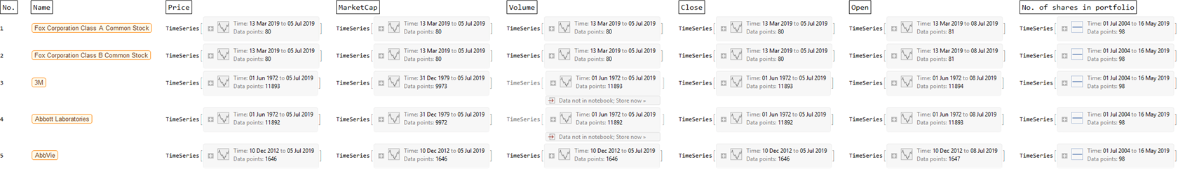
Here is an example of the finalList, with appropriate annotation.
finalListHeadings =
  Style[Framed[#], 16] & /@
   Flatten[{"No.", "Name", "Price", listOptions,
     "No. of shares in portfolio"}];
finalListwithHeadings =
  Insert[finalList, finalListHeadings, {{1}, {-1}}];

Rasterize[Take[finalListwithHeadings, 6] // TableForm,
 RasterSize -> 2400, ImageSize -> 1200]
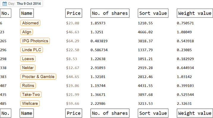
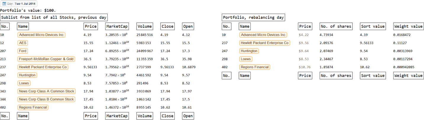
Here is an example of the portAtTime, with appropriate annotation.
portfolioAtTimeHeadings =
  Style[Framed[#], 16] & /@ {"No.", "Name", "Price", "No. of shares",
    "Sort value", "Weight value"};
dateVar = RandomChoice[listDate];
portfolioAtTime =
  Insert[portAtTime[dateVar], portfolioAtTimeHeadings, {{1}, {-1}}];

Rasterize[Column[{dateVar, Take[portfolioAtTime, 12] // TableForm}],
 RasterSize -> 1024, ImageSize -> 512]
Function callPlot[] is defined to expeditiously visualize the portfolio performance, in comparison with the Standard and Poor 500 Index if applicable (when there is no additional investment). The plot is saved in the global variable "plotVal"; and the annual rate of return is saved in the global variable "returnVal".
Function callExport[] will save the graph as a .PNG file, at the notebook's directory. Function callPlot has to be called before callExport[].
(*callPlot*)
callPlot[] := Module[{},
   frameLabel = Style[Framed[#], 12] & /@ {"Time", "Relative Value"};
   frameLable2 = {{Style[Framed["Portolio Value"], 12],
      Style[Framed["Additional Investment"], 12]}, {Style[
       Framed["Time"], 12], None}};

   stringTotal =
    ToString[
     Round[QuantityMagnitude[
       portValueTimeSeries["FirstValue"] + Total[addFundTimeSeries] -
        addFundTimeSeries["FirstValue"]], 1]];
   stringMax =
    ToString[Round[QuantityMagnitude[Max[portValueTimeSeries]], 1]];
   stringEnd =
    ToString[
     Round[QuantityMagnitude[portValueTimeSeries["LastValue"]], 1]];

   firstVal = QuantityMagnitude[addFundTimeSeries["FirstValue"]];
   regularVal = QuantityMagnitude[investAmount];
   dateVal = QuantityMagnitude[DateDifference[beginDate, endDate]]/
    timePeriod;
   lengthVal = Floor[dateVal];
   totalVal = QuantityMagnitude[portValueTimeSeries["LastValue"]];

   If[firstVal + regularVal != totalVal,

    CompoundExpression[
     sol =
      NSolve[(firstVal*(1 + interest)^lengthVal +
            regularVal ((1 + interest)^lengthVal - 1)/interest) (1 +
             interest)^(dateVal - lengthVal) == totalVal, interest,
        Reals][[1]];
     returnVal = ((1 + interest)^(365.25/timePeriod) - 1) //. sol;],

    returnVal = 0];
   stringReturn = ToString[PercentForm[returnVal, 4]];

   (*
   stringReturn=ToString[PercentForm[QuantityMagnitude[(Exp[Log[
   portValueTimeSeries["LastValue"]/Total[addFundTimeSeries]]/(
   QuantityMagnitude[DateDifference[beginDate,endDate]]/365.25)]-1;)],
   4]];

   stringTotal=StringTake[StringPadRight[ToString[portValueTimeSeries[
   "FirstValue"]+Total[addFundTimeSeries]-addFundTimeSeries[
   "FirstValue"]],9,"0"],9];
   stringMax=StringTake[StringPadRight[ToString[Max[
   portValueTimeSeries]],9,"0"],9];
   stringEnd=StringTake[StringPadRight[ToString[portValueTimeSeries[
   "LastValue"]],9,"0"],9];
   stringReturn=StringTake[StringPadRight[ToString[PercentForm[Exp[
   Log[portValueTimeSeries["LastValue"]/(portValueTimeSeries[
   "FirstValue"]+Total[addFundTimeSeries]-addFundTimeSeries[
   "FirstValue"])]/QuantityMagnitude[DateDifference[beginDate,endDate,
   "Year"]]]-1,5]],5,"0"],5];
   *)

   plotLabel =
    Style[Framed[
      StringJoin["Total investment: $", stringTotal,
       ". Annual return: ", stringReturn, "\nPortfolio value max: $",
       stringMax, "; end: $", stringEnd]], 16];

   max = Max[
     Min[QuantityMagnitude[Max[portValueTimeSeriesRatio]], 12],
     Max[sp500Ratio]];
   min = Min[
     Max[QuantityMagnitude[Min[portValueTimeSeriesRatio]], -1],
     Min[sp500Ratio]];
   plotVal = If[dailyInvest == 0,
     DateListPlot[{portValueTimeSeriesRatio, sp500Ratio,
       addFundTimeSeriesRatio}, FrameLabel -> frameLabel,
      PlotLabel -> plotLabel, PlotRange -> {Automatic, {0, max}},
      PlotStyle -> {Thick, Thick}, Joined -> {True, True, False},
      Filling -> {1 -> Axis,
        2 -> {{1}, {None,
           Directive[Opacity[0.3],
            ColorData[97, "ColorList"][[2]]]}}},
      FillingStyle -> Opacity[0.3],
      PlotLegends ->
       Placed[{"Portfolio", "SP500", "add"}, {Left, Top}],
      ImageSize -> Large],

     addFundTimeSeriesRescaled =
      addFundTimeSeries/addFundTimeSeries["LastValue"]*
       Max[portValueTimeSeries]/2;
     DateListPlot[{portValueTimeSeries, addFundTimeSeriesRescaled},
      FrameLabel -> frameLable2, PlotLabel -> plotLabel,
      PlotRange -> {Automatic, {0,
         QuantityMagnitude[Max[portValueTimeSeries]]}},
      FrameTicks -> {{Table[
          x Round[Max[portValueTimeSeries], 5]/5, {x, 0, 4}],
         Table[{x Max[portValueTimeSeries]/4,
           x addFundTimeSeries["LastValue"]/2}, {x, 1,
           3}]}, {Automatic, None}}, PlotStyle -> {Thick, Thick},
      Joined -> {True, False}, Filling -> {1 -> Axis},
      FillingStyle -> Opacity[0.3],
      PlotLegends -> Placed[{"Portfolio", "add"}, {Left, Top}],
      ImageSize -> Large]
     ]
   ];

callExport[plotVar_] := Export[
   StringJoin["plot", ToString[plotVar],
    StringPadLeft[ToString[sizePortfolio], 3, "0"],
    StringTake[ToString[optionTake], 2],
    StringPadLeft[ToString[timePeriod], 3, "0"],
    ".png"
    ]
   , plotVal];

callPlot[]
Hold[callExport[]];
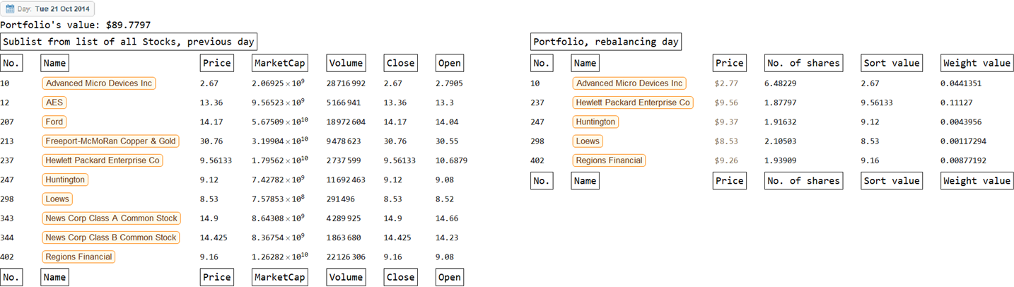
V. Explicit quality-control: checking the model manually
The model was explicitly checked to assure that it does what it is designed to do, given appropriate input data. The quality-control process is readily available using the following block of code. (Again, the sort value and weight value are derived from the day immediately before, not the current day of portfolio balancing.)
timePeriod = 112;
sizePortfolio = 5;
taxRate = 0.4;
initialInvest = 100.00;
dailyInvest = 0.00;
optionWholeShare = False;

beginDate = DateObject["2014-07-01"];
endDate = DateObject["2019-07-01"];

funcSort[x1_, x2_, x3_, x4_, x5_] := x1;
funcWeight[x1_, x2_, x3_, x4_, x5_] := (2 Abs[x5 - x4])/(x5 + x4);
optionEqualWeight = False;

callFunc[];

listDate;
listIndexTest =
  Flatten[Table[portAtTime[listDate[[q]]][[All, 1]], {q, 1, 10}]];

portfolioAtTimeHeadings =
  Style[Framed[#], 16] & /@ {"No.", "Name", "Price", "No. of shares",
    "Sort value", "Weight value"};
finalListHeadings =
  Style[Framed[#], 16] & /@
   Flatten[{"No.", "Name", "Price", listOptions}];

For[h = 1, h <= 2, h++,
 col1x = MapAt[QuantityMagnitude[#[DatePlus[listDate[[h]], -1]]] &,
   Select[masterThread, MemberQ[listIndexTest, #[[1]]] &], {All,
    Table[n, {n, 3, Length[listOptions] + 3}]}];
 col1 = Insert[col1x, finalListHeadings, {{1}, {-1}}];

 col2x = portAtTime[listDate[[h]]];
 col2 = Insert[col2x, portfolioAtTimeHeadings, {{1}, {-1}}];

 Rasterize[TableForm[{
     Rasterize[listDate[[h]]],
     Style[
      StringJoin["Portfolio's value: $",
       ToString[QuantityMagnitude[portValue[listDate[[h]]]]]], 16],

     {Style[Framed["Sublist from list of all Stocks, previous day"],
       16],
      "      ",
      Style[Framed["Portfolio, rebalancing day"], 16]},

     {col1 // TableForm,
      "      ",
      col2 // TableForm}
     }, TableAlignments -> {Left, Top}],
   RasterSize -> 2048, ImageSize -> 1024] // Print;
 ]
VI. Analysis of investment strategies
Since market conditions vary with time, the investment strategies are evaluated and compared using the same set of initial inputs, which is prescribed to best represents the current market conditions:
The function reEvaluateFunc[] simplifies the model's implementation, providing both the graph of the portfolio's performance and the annual return.
    taxRate = 0.4;
    initialInvest = 100.00;
    dailyInvest = 0.00;
    optionWholeShare = False;

    beginDate = DateObject["2014-07-01"];
    endDate = DateObject["2019-07-01"];

    reEvaluateFunc[sizePortfolioVar_, optionTakeVar_, timePeriodVar_,
       export_] :=
      Module[{o = optionTakeVar, t = timePeriodVar, s = sizePortfolioVar,
        ex = export},
       timePeriod = t;
       sizePortfolio = s;
       optionTake = o;

       callFunc[];
       callPlot[];
       If[ex == True, callExport[]];

       {plotVal, returnVal}

       ];
a) The sorted and weighted by price strategy
The sorted and weighted by price portfolio is one of the most common and simple strategies. This strategy results in equal number of shares for the stocks in portfolio (almost equal actually, since price of the day before adjustment is used as weight, but portfolio value is distributed to price of adjustment day).
funcSort[x1_, x2_, x3_, x4_, x5_] := x1 ;
funcWeight[x1_, x2_, x3_, x4_, x5_] := x1;
optionEqualWeight = False;

plota11 = reEvaluateFunc[10, "high", 056, False][[1]];
plota21 = reEvaluateFunc[10, "high", 014, False][[1]];
plota31 = reEvaluateFunc[60, "high", 056, False][[1]];
plota41 = reEvaluateFunc[60, "high", 014, False][[1]];

plota12 = reEvaluateFunc[10, "mid", 056, False][[1]];
plota22 = reEvaluateFunc[10, "mid", 014, False][[1]];
plota32 = reEvaluateFunc[60, "mid", 056, False][[1]];
plota42 = reEvaluateFunc[60, "mid", 014, False][[1]];

plota13 = reEvaluateFunc[10, "low", 056, False][[1]];
plota23 = reEvaluateFunc[10, "low", 014, False][[1]];
plota33 = reEvaluateFunc[60, "low", 056, False][[1]];
plota43 = reEvaluateFunc[60, "low", 014, False][[1]];

k = 32;
tabLabel =
  Style[Framed[
    "Portfolio's value, comparing to S&P500\nSorted and Weighted by \
Price"], 1.25 k];
row1 = Style[Framed["Base Case:\nperiod 56\nsize 10"], k];
row2 = Style[Framed["\[DownArrow]period 14\nsize 10"], k];
row3 = Style[Framed["period 56\n\[UpArrow]size 60"], k];
row4 = Style[Framed["\[DownArrow]period 14\n\[UpArrow]size 60"], k];
col1 = Style[Framed["Largest Stocks"], k];
col2 = Style[Framed["Middle Stocks"], k];
col3 = Style[Framed["Smallest Stocks"], k];

plotLista = {
   {"", col1, col2, col3},
   {row1, plota11, plota12, plota13},
   {row2, plota21, plota22, plota23},
   {row3, plota31, plota32, plota33},
   {row4, plota41, plota42, plota43},
   {"", tabLabel, SpanFromLeft, SpanFromLeft}};
Rasterize[TableForm[plotLista, TableAlignments -> Center]]
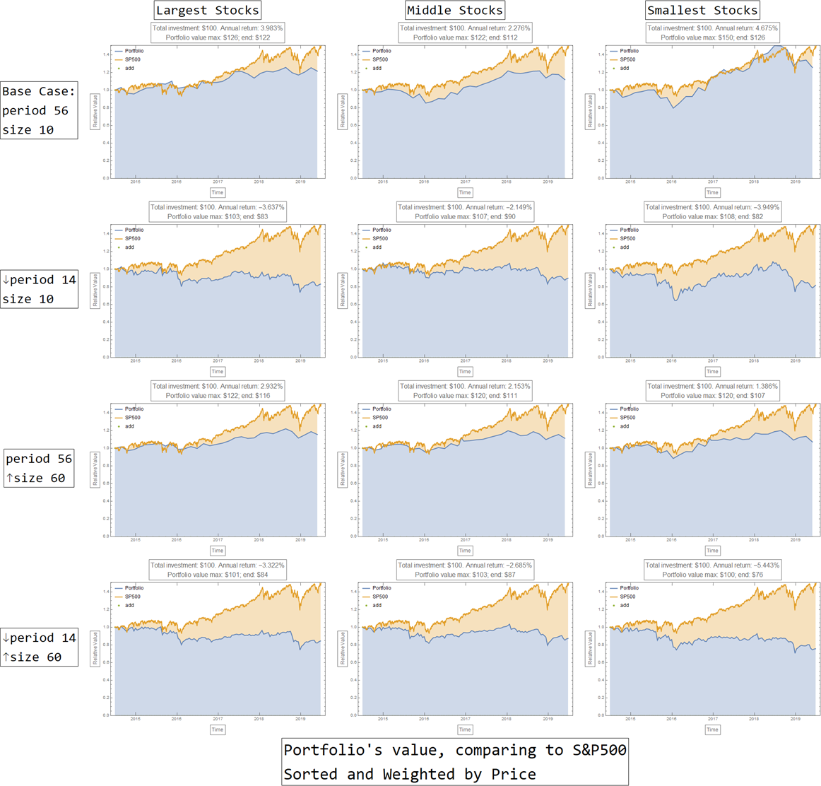
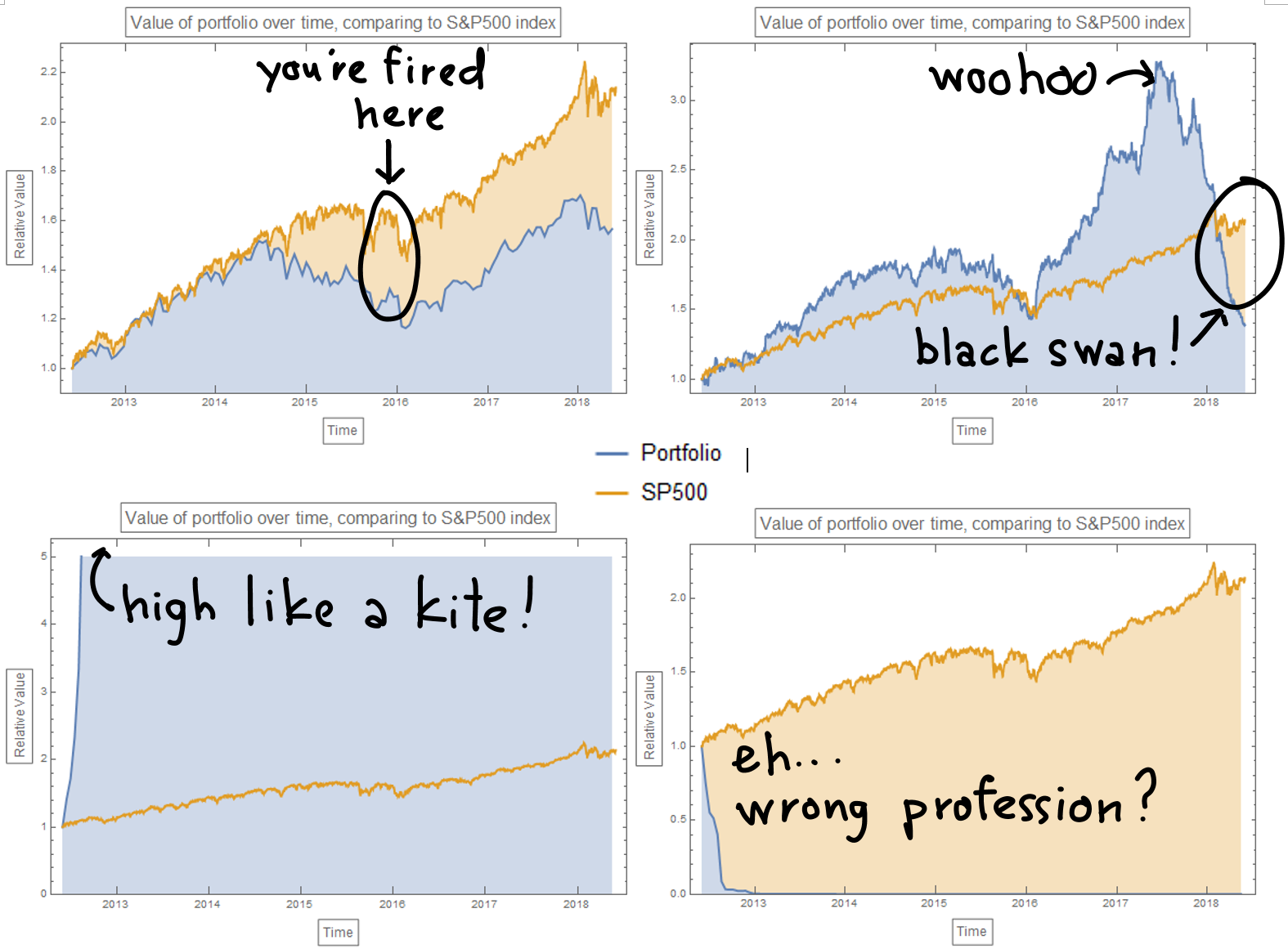
For this simple investment strategy:
a longer period of adjustment - a less frequent portfolio rebalancing schedule would generally yield a significantly better return (comparing row 1 and row 2, row 3 and row 4).
independent of how the stocks are chosen (largest, middle, and smallest, with respect to the sorting criteria), the size of the portfolio does not seem to affect portfolio's performance: gaining portfolios remains gaining, and losing portfolios remains losing (comparing row 1 and row 3, row 2 and row 4).
Among the twelves scenarios investigated for this investment strategy, the scenario of choosing the smallest stocks and holding them for a longer period of time seems to be nearly as profitable as passive investing in SP500 Index, yielding a 1.50 times profit, corresponding to an annual return of 4.68%.
b) The sorted by price, equally weighted strategy
This investment strategy is very similar to its cousin above: instead of equal number of share, each stock in the portfolio receive an equal amount of investment.
funcSort[x1_, x2_, x3_, x4_, x5_] := x1;
funcWeight[x1_, x2_, x3_, x4_, x5_] := x1;
optionEqualWeight = True;

plotb11 = reEvaluateFunc[10, "high", 056, False][[1]];
plotb12 = reEvaluateFunc[10, "mid", 056, False][[1]];
plotb13 = reEvaluateFunc[10, "low", 056, False][[1]];

k = 32;
tabLabel =
  Style[Framed[
    "Portfolio's value, comparing to S&P500\nSorted by Price, Equally \
Weighted"], 1.25 k];
row1 = Style[Framed["period 56\nsize 10"], k];
col1 = Style[Framed["Largest Stocks"], k];
col2 = Style[Framed["Middle Stocks"], k];
col3 = Style[Framed["Smallest Stocks"], k];

plotListb = {
   {"", col1, col2, col3},
   {row1, plotb11, plotb12, plotb13},
   {"", tabLabel, SpanFromLeft, SpanFromLeft}};
Rasterize[TableForm[plotListb, TableAlignments -> Center]]
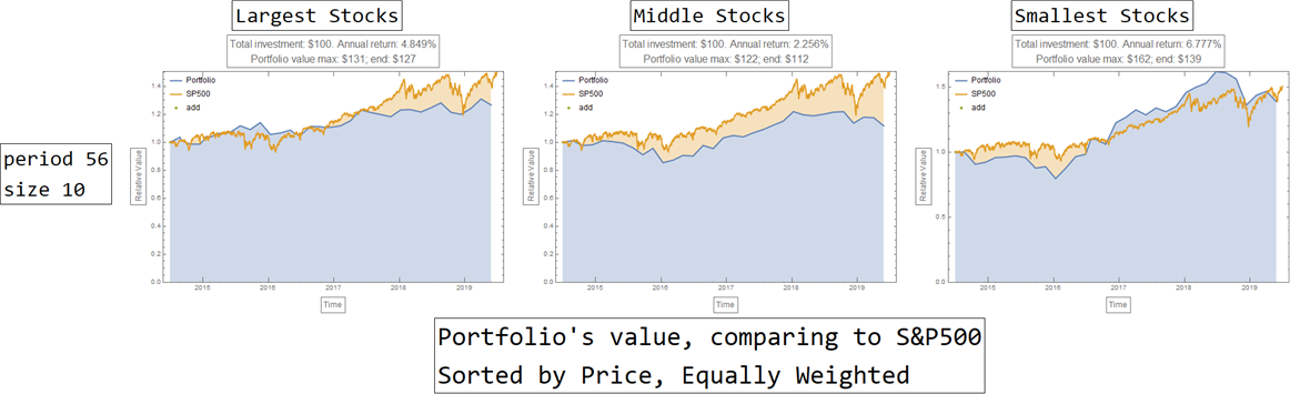
The sorted by price, equally weighted strategy performs a bit better comparing to its relative (sorted and weighted by price). Nevertheless, it remains inferior to passively investing in SP500 Index: it only gives an annual return of 6.78%, similar to SP500.
c) The sorted by volume, weighted by market capitalization strategy
funcSort[x1_, x2_, x3_, x4_, x5_] := x3;
funcWeight[x1_, x2_, x3_, x4_, x5_] := x2;
optionEqualWeight = False;

plotc11 = reEvaluateFunc[10, "high", 056, False][[1]];
plotc12 = reEvaluateFunc[10, "mid", 056, False][[1]];
plotc13 = reEvaluateFunc[10, "low", 056, False][[1]];

k = 32;
tabLabel =
  Style[Framed[
    "Portfolio's value, comparing to S&P500\nSorted by Volume, \
Weighted by Market Cap."], 1.25 k];
row1 = Style[Framed["period 56\nsize 10"], k];
col1 = Style[Framed["Largest Stocks"], k];
col2 = Style[Framed["Middle Stocks"], k];
col3 = Style[Framed["Smallest Stocks"], k];

plotListc = {
   {"", col1, col2, col3},
   {row1, plotc11, plotc12, plotc13},
   {"", tabLabel, SpanFromLeft, SpanFromLeft}};
Rasterize[TableForm[plotListc, TableAlignments -> Center]]
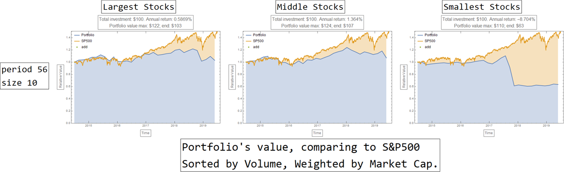
This strategy is abysmal: it manages to earn significantly less than the SP500 Index, or even lose money over time. However, it indicates perhaps a relevant strategy of shorting (selling) these portfolios - instead of longing (buying) them - might be profitable.
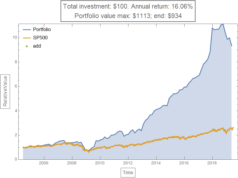
d) The sorted and weighted by market capitalization strategy
funcSort[x1_, x2_, x3_, x4_, x5_] := x2;
funcWeight[x1_, x2_, x3_, x4_, x5_] := x2;
optionEqualWeight = False;

beginDate = DateObject["2014-07-01"];
endDate = DateObject["2019-07-01"];
plotd11 = reEvaluateFunc[10, "high", 056, False][[1]];
plotd12 = reEvaluateFunc[10, "mid", 056, False][[1]];
plotd13 = reEvaluateFunc[10, "low", 056, False][[1]];

beginDate = DateObject["2009-07-01"];
endDate = DateObject["2019-07-01"];
plotd21 = reEvaluateFunc[10, "high", 056, False][[1]];
plotd22 = reEvaluateFunc[10, "mid", 056, False][[1]];
plotd23 = reEvaluateFunc[10, "low", 056, False][[1]];

beginDate = DateObject["2004-07-01"];
endDate = DateObject["2019-07-01"];
plotd31 = reEvaluateFunc[10, "high", 056, False][[1]];
plotd32 = reEvaluateFunc[10, "mid", 056, False][[1]];
plotd33 = reEvaluateFunc[10, "low", 056, False][[1]];

k = 32;
tabLabel =
  Style[Framed[
    "Portfolio's value, comparing to S&P500\nSorted and Weighted by \
Market Capitalization"], 1.25 k];
row1 = Style[Framed["period 56\nsize 10\n5 years"], k];
row2 = Style[Framed["10 years"], k];
row3 = Style[Framed["15 years"], k];
col1 = Style[Framed["Largest Stocks"], k];
col2 = Style[Framed["Middle Stocks"], k];
col3 = Style[Framed["Smallest Stocks"], k];

plotListd = {
   {"", col1, col2, col3},
   {row1, plotd11, plotd12, plotd13},
   {row2, plotd21, plotd22, plotd23},
   {row3, plotd31, plotd32, plotd33},
   {"", tabLabel, SpanFromLeft, SpanFromLeft}};
Rasterize[TableForm[plotListd, TableAlignments -> Center]]
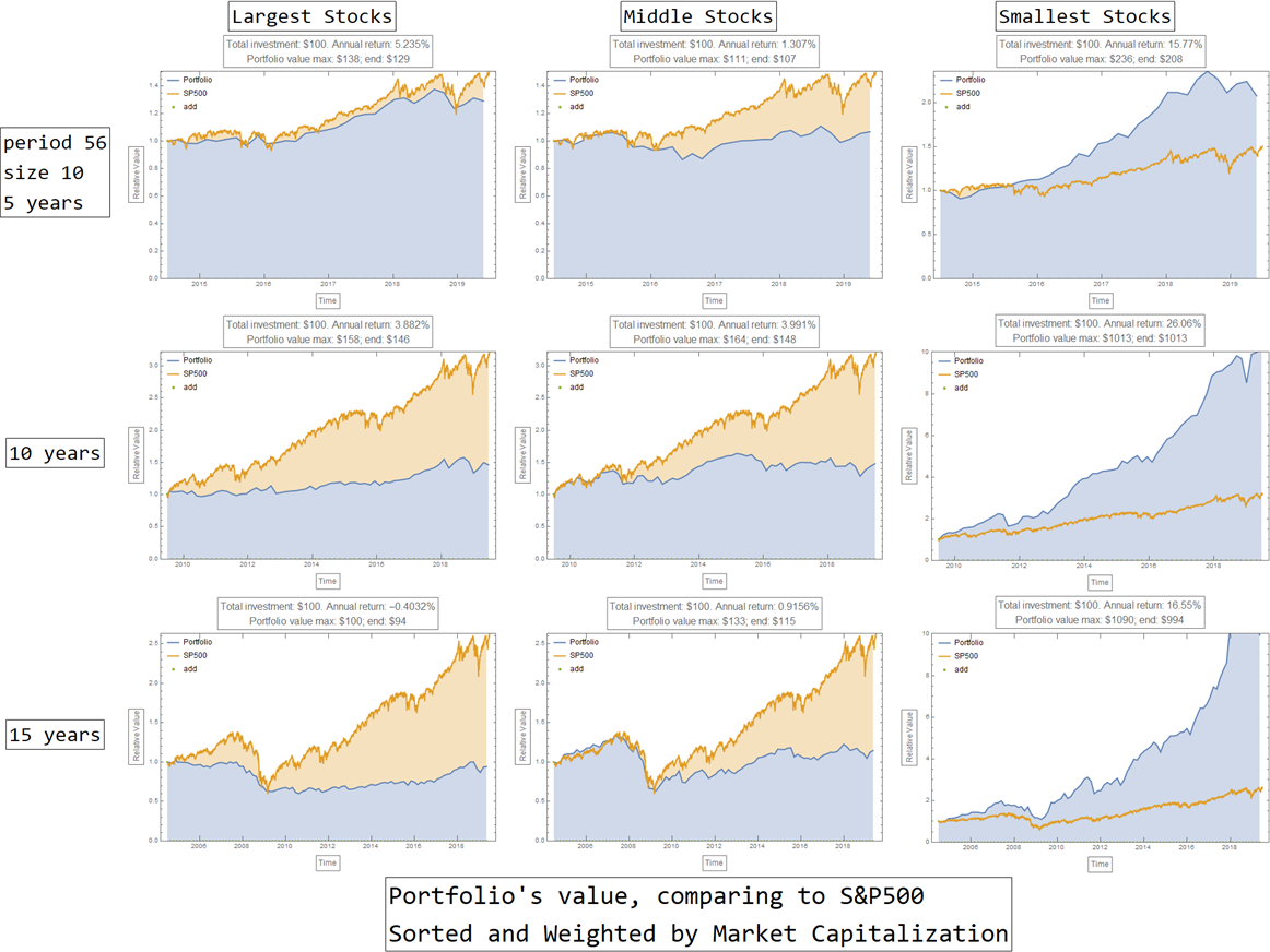
Theoretically, this strategy looks wonderful for stocks of small market capitalization: an annual return of 15.8% is impressive. It consistently performs significantly better than SP500 Index over different time frame (data not shown): 5, 10, 15 years till today. However, the strategy's consistent performance instills doubts of systematic errors, either in the model itself or in the input data (as discussed in the next section).
VII. Discussion
A versatile computation model for portfolio's performance was derived, which allows investment strategies to be analyzed and quantified. The model shows that a less frequently adjusted portfolio seems to perform better, supporting the buy-and-hold tactic. The model also indicate that the size of the portfolio does not exert a strong effect on the strategy's overall performance.
Generally, the model suggests that portfolios of small stocks (with respect to the sorting criteria) seem to outperform portfolios of larger stocks.
There are two know systematic errors regarding the input data, which may significantly distort the results the model provided:
The stocks in Entity Class SP500 are the current components of the Standard and Poor 500 Index. Since the composition of SP500 changes over time, some of these stocks might not be included in the index until recently. As SP500 signifies large, successful companies, choosing the stocks that would be in SP500 in the future, but not at the time of portfolio rebalancing, would result in survivor bias. The same is true for excluding stocks that were in SP500 in the past, but is no longer a component of the index (for example, Enron). This survivor bias is expected to be much less significant with recent time period (e.g. past 5 years), comparing to more distant time period (e.g. past 10, 15 years).
At least one stock received insufficient property, which affects how the stocks are chosen and weighed: as of 2019-07-28, the FinancialData[] call for Loews, "NYSE:L", only provide a timeseries of price up to 2013-11-05, which means price after that day is erroneous (due to missing value and interpolation), as shown in the block of codes below.
FinancialData[Entity["Financial", "NYSE:L"], "Price"]
FinancialData[Entity["Financial", "NYSE:L"], "Price", All]["LastValue"]
FinancialData[Entity["Financial", "NYSE:L"], "Price",
              {2013-01-01, 2019-07-01}]
Just For Fun