Disclaimer
?This computational notebook is not for commercial purposes. ?The calculation only serves as an additional reference for medical doctors and specialists. Any liability, including any liability for negligence, for any loss or damage arising from reliance on this computational notebook, is expressly excluded.
I. Abstract
Plasma concentration of pharmaceuticals helps doctors and medical professionals decide the appropriate treatment course for patients. Although it is essential and conceptually simple, the theoretical plasma drug concentration are not readily accessible due to a lack of computational shortcuts, which undermines the prescription of correct dosing amount and schedule. Hence, several computational models were derived to determine the plasma drug concentration and its associated concentration-versus-time-graph, in both uniform and varied dosing amount/schedule, as well as in different order of reactions. These computational models specify certain sets of conditions to keep plasma drug concentration within therapeutics range, enabling the prescription of more suitable, tailored dose amount and schedule.
II. Introduction
Plasma (serum) drug concentration is an essential aspect of treatment therapy: because plasma drug concentration must remains within therapeutic range [Dash] above minimum effective dose and below lethal dose, it guides the dosage amount and frequency. Even though the theoretical frameworks to determine plasma drug concentration exist [1], [2], hardly any medical professionals use these computations to decide the appropriate/tailored drug regime (generally, medications are prescribed based on convention and experience, by tried-and-true methods [3]: if a certain base drug regime does not work, either the dosing amount needs to be increased, or different medications should be used. For example, it is a common practice to apply more pain relievers when patients still experience discomfort).
Despite their inclusion in core medical curriculum, the frameworks to determine plasma drug concentration based on reaction kinetics were not routinely used, probably because there is no convenient, easily accessible computational shortcuts. The frameworks are conceptually simple, but potentially challenging in calculation: they requires solving the differential equation $$\frac{\mathbb{d}y}{\mathbb{d}t}=-r y^n$$ with drug-dependent constants $r$ for reaction rate and $n$ for reaction order, and recursively applying the formula each instant the medication is introduced. [4], [3], [6]
The vast majority of medications follow the first order reaction: when n = 1, solving the differential equation $\frac{\mathbb{d}y}{\mathbb{d}t}=-r y$ gives solution $y(t)=y_0 \mathbb{e}^{-r t}$, with constant half-life $t_{0.5}=\frac{Log(2)}{r}$. The computation techniques to calculate and visualize plasma concentration of drugs that follow the first order reaction were compiled [1], [4], although they are not yet distributed on public domain (the internet). Due to the rare occurrence of pharmaceuticals of zeroth order (salicylates, alcohols: methanol, ethanol [4], [5]), second order (aspirin [6]), and higher orders - it is not known whether the plasma drug concentration of medication following these rare reaction orders has been investigated.
Hence, several computational models to calculate plasma drug concentration were derived: for the simplest case of zeroth order, the most common case of first order, and the general case of irregular dose amount-schedule with non-specified order.
III. The simplest case: uniform dosing at regular interval of drugs that follow zeroth order reaction
For zeroth order reaction $(n = 0)$, the differential equation $\frac{\mathbb{d}y}{\mathbb{d}t}=-r y^0 = -r$ gives solution $y(t)=y_0 - r t$, which is represented by the function funcZero[time t, initial value y0, rate constant r] below.
ClearAll["Global`*"];
funcZeroth[t_, y0_, r_] :=
  DSolveValue[{y'[x] == -r, y[0] == y0}, y[x], x] /. {x -> t};
funcZeroth[t, y0, r]
Assume the variables for
- uniform dosing is drugDose,
- regular interval is drugInterval, and
- reaction rate is drugRate.
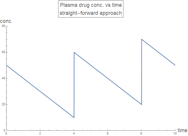
A straight-forwards approach is attempted, for the first three doses:
rxnZerothDraft1[time_, drugDose_, drugInterval_, drugRate_] :=
  Piecewise[{
    {0, time < 0},
    {funcZeroth[time, drugDose, drugRate], 0 <= time <  drugInterval},
    {funcZeroth[time - drugInterval,
      drugDose + funcZeroth[drugInterval, drugDose, drugRate],
      drugRate], drugInterval <= time <  2 drugInterval},
    {funcZeroth[time - 2 drugInterval,
      drugDose +
       funcZeroth[drugInterval,
        drugDose + funcZeroth[drugInterval, drugDose, drugRate],
        drugRate], drugRate], 2 drugInterval <= time <  3 drugInterval}
    }];

plotLabel1 =
  Style[Framed[
    "Plasma drug conc. vs time\nstraight-forward approach"], 16];
axesLabel = {Style["time", 16], Style["conc.", 16]};
Plot[rxnZerothDraft1[t, 50, 4, 10], {t, 0, 10},
 PlotLabel -> plotLabel1, AxesLabel -> axesLabel,
 PlotRange -> {{0, 10}, {0, 80}}, PlotStyle -> Thick,
 ExclusionsStyle -> {{Thick, ColorData[97, "ColorList"][[1]]}, None},
 ImageSize -> Large]
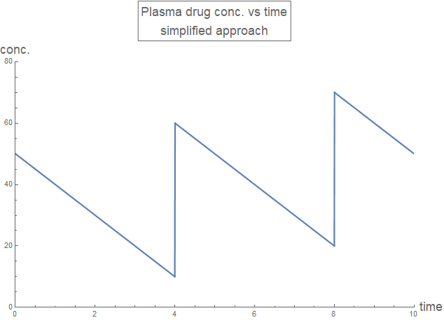
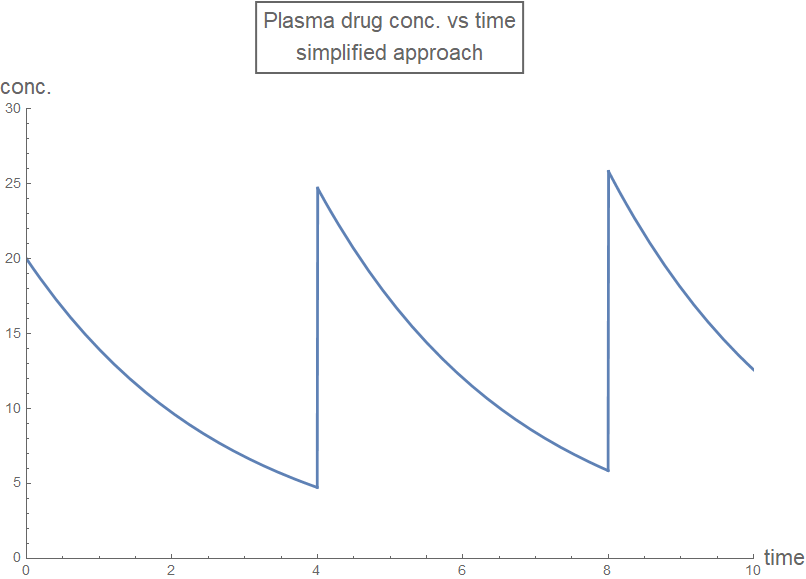
With some algebra (using pen and paper), the recursive applications of funcZeroth[time t, initial value y0, rate constant r] at each dosing instant can be simplified:
rxnZerothDraft2[time_, drugDose_, drugInterval_, drugRate_] :=
  Piecewise[{
    {0, time < 0},
    {drugDose - drugRate*time , 0 <= time <  drugInterval},
    {2 drugDose - drugRate*time,
     drugInterval <= time <  2 drugInterval},
    {3 drugDose - drugRate*time,
     2 drugInterval <= time <  3 drugInterval}
    }];

plotLabel2 =
  Style[Framed["Plasma drug conc. vs time\nsimplified approach"], 16];
Plot[rxnZerothDraft2[t, 50, 4, 10], {t, 0, 10},
 PlotLabel -> plotLabel2, AxesLabel -> axesLabel,
 PlotRange -> {{0, 10}, {0, 80}}, PlotStyle -> Thick,
 ExclusionsStyle -> {{Thick, ColorData[97, "ColorList"][[1]]}, None},
 ImageSize -> Large]
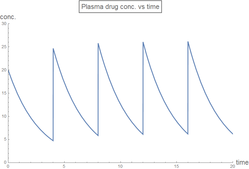
Hence, for the uniform dosing at regular interval of drugs that follow zeroth order reaction, the plasma drug concentration is derived in the function rxnZeroth[time, drugFirstDose, drugDose, drugInterval, drugRate] below. The initial dose is separated to allow the adjustment of minimum plasma drug concentration, which would be apparent later.
rxnZeroth[time_, drugFirstDose_, drugDose_, drugInterval_,
  drugRate_] :=
 Module[{t = time, dose1 = drugFirstDose, dose = drugDose,
   rate = drugRate, interval = drugInterval, numPeriod},
  numPeriod = Ceiling[t/interval];
  Piecewise[Join[
    {{0, t < 0}},
    {{Max[dose1 - rate*t, 0], 0 <= t < interval}},
    Table[{Max[dose1 + (k - 1) dose - rate*t, 0], (k - 1) interval <=
       t <= k interval}, {k, 2, numPeriod}],
    {{numPeriod*dose - rate*t, numPeriod*interval <= t}}
    ]]]

plotLabel3 = Style[Framed["Plasma drug conc. vs time"], 16];
Plot[rxnZeroth[t, 50, 50, 4, 10], {t, 0, 40},
 PlotRange -> {{0, 40}, {0, 150}}, PlotLabel -> plotLabel3,
 AxesLabel -> axesLabel, PlotStyle -> Thick,
 ExclusionsStyle -> {{Thick, ColorData[97, "ColorList"][[1]]}, None},
 ImageSize -> Large]
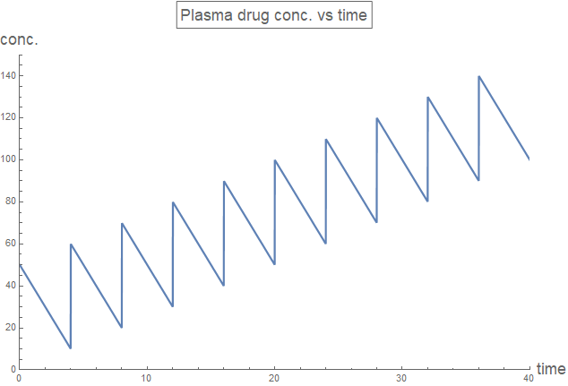
The plasma drug concentration oscillates during the course of treatment. However, the maximum and minimum concentration remain stable only when drugDose=drugRate*drugInterval. Additionally, the initial dose has to be larger than the regular doses, in order to bring the stable minimum concentration above zero.
plotRange = {{0, 30}, {0, 150}};
plotStyle[n_] := {Thick, ColorData[97, "ColorList"][[n]]};
plotLabel4 =
  Style[Framed[
    "Plasma drug conc. vs time of different dosing regime\nshowing \
stable min and max conc. when dose = rate * interval"], 16];
plotLegend =
  LineLegend[{{ColorData[97, "ColorList"][[1]], Dashed},
    ColorData[97, "ColorList"][[2]], {ColorData[97, "ColorList"][[3]],
      DotDashed}},
   {"dose < rate * interval", "dose = rate * interval",
    "dose > rate * interval"}];

plot01 = Plot[rxnZeroth[t, 105, 50, 6, 10], {t, 0, 30},
   PlotRange -> plotRange, PlotStyle -> Join[plotStyle[1], {Dashed}],
   ExclusionsStyle -> {plotStyle[1], None},
   PlotLegends -> Placed[plotLegend, Right], ImageSize -> Large];
plot02 = Plot[rxnZeroth[t, 105, 60, 6, 10], {t, 0, 30},
   PlotRange -> plotRange, PlotStyle -> Join[plotStyle[2]],
   ExclusionsStyle -> {plotStyle[2], None}];
plot03 = Plot[rxnZeroth[t, 105, 70, 6, 10], {t, 0, 30},
   PlotRange -> plotRange,
   PlotStyle -> Join[plotStyle[3], {DotDashed}],
   ExclusionsStyle -> {plotStyle[3], None}];
Show[plot01, plot02, plot03, PlotRange -> plotRange,
 PlotLabel -> plotLabel4, AxesLabel -> axesLabel]
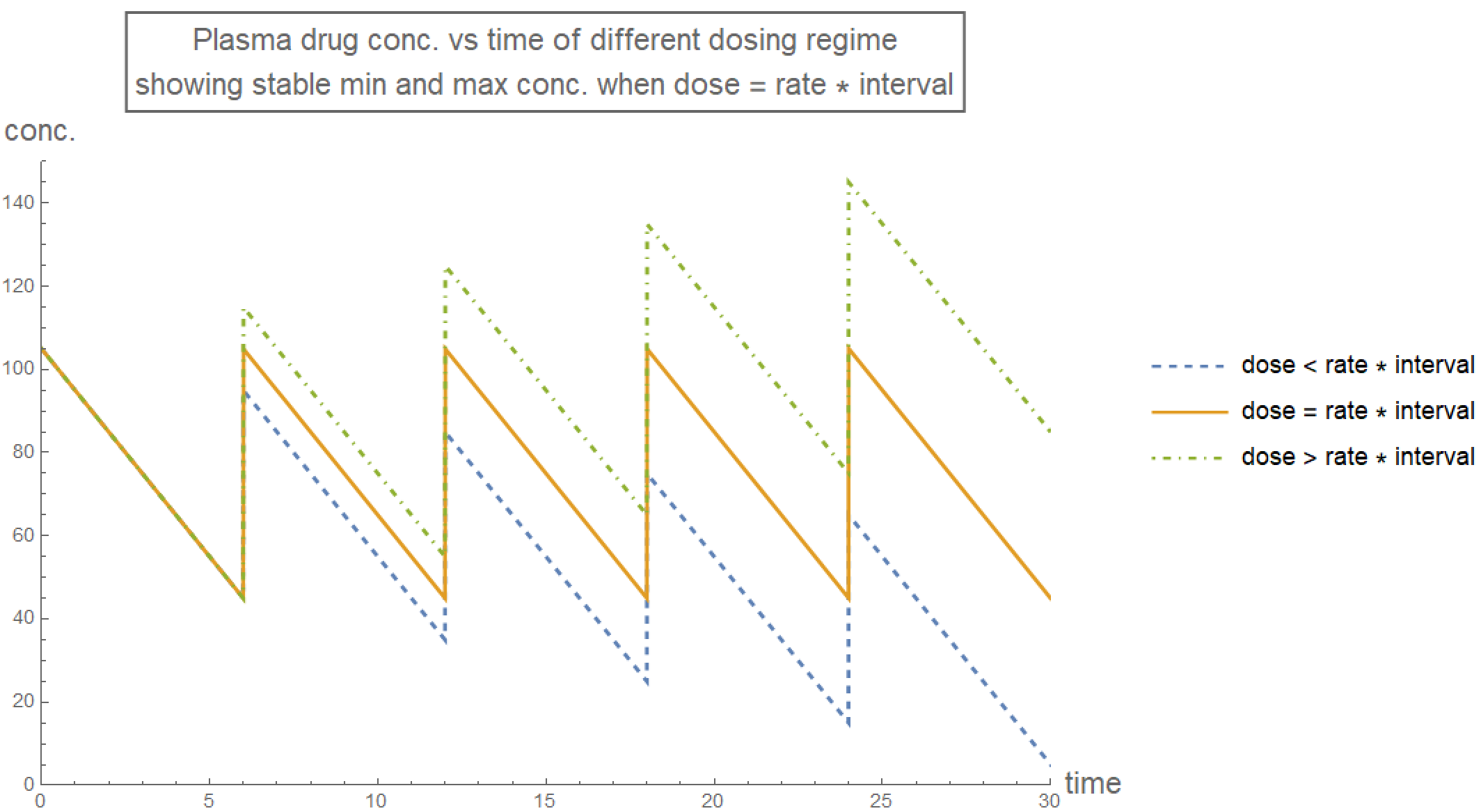
Since plasma drug concentration must be within the therapeutic range, the stable condition for its maximum and minimum values suggest a suitable treatment regime for medication of first order kinetics:
- initial dose - rate * interval > minimum effective dose,
- dose + (initial dose - rate * interval) < lethal dose
IV. The common case: uniform dosing at regular interval of drugs that follow first order reaction
For first order reaction $(n = 1)$, the differential equation $\frac{\mathbb{d}y}{\mathbb{d}t}=-r y$ gives solution $y(t)=y_0 \mathbb{e}^{-r t}$, which is represented by the function funcFirst[time t, initial value y0, rate constant r] below:
ClearAll["Global`*"];
funcFirst[t_, y0_, r_] :=
  DSolveValue[{y'[x] == -r y[x], y[0] == y0}, y[x], x] /. {x -> t};
funcFirst[t, y0, r]
Similarly, assume the variables for
- uniform dosing is drugDose,
- regular interval is drugInterval, and
- reaction rate is drugRate.
A straight-forwards approach is attempted, for the first three doses:
rxnFirstDraft1[time_, drugDose_, drugInterval_, drugRate_] :=
  Piecewise[{
    {0, time < 0},
    {funcFirst[time, drugDose, drugRate], 0 <= time <  drugInterval},
    {funcFirst[time - drugInterval,
      drugDose + funcFirst[drugInterval, drugDose, drugRate],
      drugRate], drugInterval <= time <  2 drugInterval},
    {funcFirst[time - 2 drugInterval,
      drugDose +
       funcFirst[drugInterval,
        drugDose + funcFirst[drugInterval, drugDose, drugRate],
        drugRate], drugRate], 2 drugInterval <= time <  3 drugInterval}
    }];

plotLabel1 =
  Style[Framed[
    "Plasma drug conc. vs time\nstraight-forward approach"], 16];
axesLabel = {Style["time", 16], Style["conc.", 16]};
Plot[rxnFirstDraft1[t, 20, 4, 0.36], {t, 0, 10},
 PlotLabel -> plotLabel1, AxesLabel -> axesLabel,
 PlotRange -> {{0, 10}, {0, 30}}, PlotStyle -> Thick,
 ExclusionsStyle -> {{Thick, ColorData[97, "ColorList"][[1]]}, None},
 ImageSize -> Large]

With some algebra (again, using pen and paper), the recursive applications of funcFirst[time t, initial value y0, rate constant r] at each dosing instant can be drastically simplified:
rxnFirstDraft2[time_, drugDose_, drugInterval_, drugRate_] :=
 Module[{t = time, dose = drugDose, rate = drugRate,
   interval = drugInterval, k},
  k = Exp[-rate*interval];
  Piecewise[{
    {0, t < 0},
    {dose Exp[-rate t], 0 <= t < interval},
    {dose ( k + 1) Exp[-rate (t - interval)],
     interval <= t < 2 interval},
    {dose (k^2 + k + 1) Exp[-rate (t - 2 interval)],
     2 interval <= t < 3 interval},
    {dose (k^3 + k^2 + k + 1) Exp[-rate (t - 3 interval)],
     3 interval <= t < 4 interval},
    {dose (k^4 + k^3 + k^2 + k + 1) Exp[-rate (t - 4 interval)],
     4 interval <= t < 5 interval},
    {dose (k^5 + k^4 + k^3 + k^2 + k + 1) Exp[-rate (t - 5 interval)],
      5 interval <= t < 6 interval},
    {dose (k^6 + k^5 + k^4 + k^3 + k^2 + k +
        1) Exp[-rate (t - 6 interval)], 6 interval <= t < 7 interval}
    }]
  ]

plotLabel2 =
  Style[Framed["Plasma drug conc. vs time\nsimplified approach"], 16];
Plot[rxnFirstDraft2[t, 20, 4, 0.36], {t, 0, 10},
 PlotLabel -> plotLabel2, AxesLabel -> axesLabel,
 PlotRange -> {{0, 10}, {0, 30}}, PlotStyle -> Thick,
 ExclusionsStyle -> {{Thick, ColorData[97, "ColorList"][[1]]}, None},
 ImageSize -> Large]
Hence, for the uniform dosing at regular interval of drugs that follow first order reaction, the plasma drug concentration is derived in the function rxnFirst[time, drugFirstDose, drugDose, drugInterval, drugRate] below.
rxnFirst[time_, drugDose_, drugInterval_, drugRate_] :=
 Module[{t = time, dose = drugDose, rate = drugRate,
   interval = drugInterval, numPeriod, k},
  k = Exp[-rate*interval];
  numPeriod = Floor[t/interval];
  Piecewise[Join[
    {{0, t < 0}},
    Table[{dose \!\(
\*UnderoverscriptBox[\(\[Sum]\), \(a = 0\), \(h\)]\(
\*SuperscriptBox[\(k\), \(a\)] Exp[\(-rate\) \((t -
             h\ interval)\)]\)\),
      h interval <= t < (h + 1) interval}, {h, 0, numPeriod}]
    ]]]

plotLabel3 = Style[Framed["Plasma drug conc. vs time"], 16];
Plot[rxnFirst[t, 20, 4, 0.36], {t, 0, 20},
 PlotRange -> {{0, 20}, {0, 30}}, PlotLabel -> plotLabel3,
 AxesLabel -> axesLabel, PlotStyle -> Thick,
 ExclusionsStyle -> {{Thick, ColorData[97, "ColorList"][[1]]}, None},
 ImageSize -> Large]
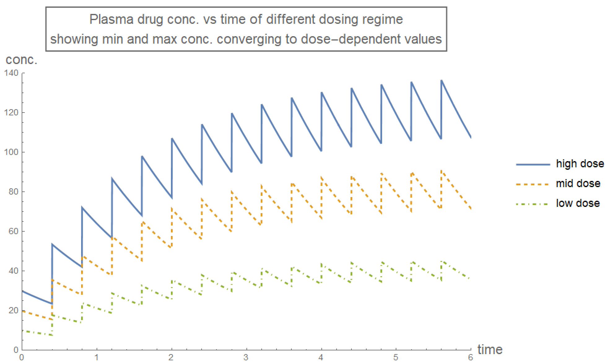
The plasma drug concentration oscillates during the course of treatment. However, the maximum and minimum concentration converge to their equilibrium level in the long-run, as determined by the function rxnFirstEquiConc[drugDose, drugInterval ,drugRate] below.
"output: {high equil. conc., low equil. conc.}";
rxnFirstEquiConc[drugDose_, drugInterval_, drugRate_] :=
  Module[{dose = drugDose, rate = drugRate, interval = drugInterval,
    k},
   k = Exp[-rate*interval];
   {dose/(1 - k), (k dose)/(1 - k)}
   ];

plotRange = {{0, 6}, {0,
    Round[rxnFirstEquiConc[30, 0.4, 0.6][[1]], 10]}};
plotLabel4 =
  Style[Framed[
    "Plasma drug conc. vs time of different dosing regime\nshowing \
min and max conc. converging to dose-dependent values"], 16];
plotLegend =
  LineLegend[{{ColorData[97, "ColorList"][[
      1]]}, {ColorData[97, "ColorList"][[2]],
     Dashed}, {ColorData[97, "ColorList"][[3]], DotDashed}}];

Plot[{rxnFirst[t, 30, 0.4, 0.6], rxnFirst[t, 20, 0.4, 0.6],
  rxnFirst[t, 10, 0.4, 0.6]}, {t, 0, 6}, PlotLabel -> plotLabel4,
 AxesLabel -> axesLabel, PlotRange -> plotRange,
 PlotStyle -> {Thick, {Thick, Dashed}, {Thick, DotDashed}},
 PlotLegends -> {"high dose", "mid dose", "low dose"},
 ImageSize -> Large]
Since plasma drug concentration must be within the therapeutic range, its dose-dependent long-run maximum and minimum values suggest a suitable treatment regime for medication of first order kinetics:
- $\frac{\mathbb{e}^{-\text{rate interval}}}{1-\mathbb{e}^{-\text{rate interval}}} \text{dose} > \text{minimum effective dose}$
- $\frac{1}{1-\mathbb{e}^{-\text{rate interval}}} \text{dose} < \text{maximum effective dose}$
Furthermore, the plasma drug concentration should ideally converge to its long-run profile as fast as possible, which means $1-\mathbb{e}^{-\text{rate interval}}$ should be close to 1. Also, the fluctuation between maximum and minimum concentrations should ideally be as small as possible, which means $\mathbb{e}^{-\text{rate interval}}$ should be close to 1. The two constraints on $1-\mathbb{e}^{-\text{rate interval}}$ and \mathbb{e}^{-\text{rate interval}} reflect the trade-off between fast convergence and small fluctuation when uniform dosing amount is applied. This trade-off can be avoided with a larger initial dose to immediately bring the plasma drug concentration profile to equilibrium: $\text{initial dose} = \frac{\text{dose}}{1-\mathbb{e}^{-\text{rate interval}}}$.
V. The general case: irregular dosing amounts and intervals of drugs that follow any order reaction
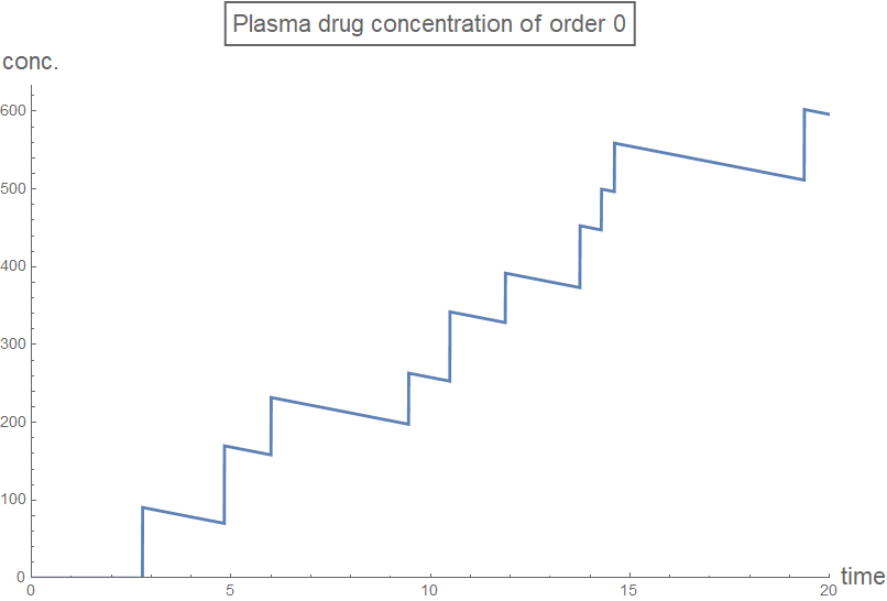
For the general case of non-specific reaction order, irregular drug dosing amount and schedule, only the straight-forward brute force method is possible. Assume the variables for - reaction rate is drugRate, - reaction order is drugOrder
The function rxnGeneral[drugTime, drugTimeAmountList, drugRate, drugOrder] was derived to compute the plasma drug concentration of a drug with know drugRate and drugOrder. The function rxnGeneral takes input from a sorted list of dose schedule and amount (sorted by time/schedule - the instant the dose amount is introduced), splits that list into two list: timeList containing the dose time only, and amountList containing the dose amount only.
First, the function rxnGeneral calls a sub-function funcOrder, which solves the kinetic differential equation $\frac{\mathbb{d}y}{\mathbb{d}t}=-r y^n$. The function rxnGeneral would run faster if DSolve does not have to be re-evaluated each time funcOrder is called, for example, set FuncOrder[A,t,]=Assuming[{Element[A,Reals],A>0,x>0},DSolveValue[{y'[x]==-rate y[x]^order,y[0]==A},y[x],x]/.{x-> t}], i.e. using "=" instead of ":=". However, since there are multiple possible solution branches with the symbolic solution, it is necessary that the DSolve has to be re-applied with each new set of dose timing and amount input.
Then, the function rxnGeneral defines a recursive sequence of plasma drug concentration just before each new dose, and uses this sequence to return a piecewise function of plasma drug concentration during the whole treatment course.
ClearAll["Global`*"];
rxnGeneral[drugTime_, drugTimeAmountList_List, drugRate_,
  drugOrder_: 1] :=
 Module[{time = drugTime, timeAmountList = drugTimeAmountList,
   rate = drugRate, order = drugOrder, amountList, timeList,
   funcOrder, listLength, sequenceAmountBeforeEachJump},
  listLength = Length[timeAmountList];
  amountList = timeAmountList[[All, 2]];
  timeList = timeAmountList[[All, 1]];

  funcOrder[A_, t_, r_, n_] :=
   DSolveValue[{y'[x] == -r y[x]^n, y[0] == A}, y[x], x] /. {x -> t};

  sequenceAmountBeforeEachJump[1] = 0;
  sequenceAmountBeforeEachJump[n_] :=
   sequenceAmountBeforeEachJump[n] =
    funcOrder[
     sequenceAmountBeforeEachJump[n - 1] + amountList[[n - 1]],
     timeList[[n]] - timeList[[n - 1]], rate, order];

  Piecewise[Join[
    {{0, time < timeList[[1]]}},
    Table[{funcOrder[
       sequenceAmountBeforeEachJump[k] + amountList[[k]],
       time - timeList[[k]], rate, order],
      timeList[[k]] <= time < timeList[[k + 1]]},
     {k, 1, listLength - 1}],
    {{funcOrder[
       sequenceAmountBeforeEachJump[listLength] +
        amountList[[listLength]], time - timeList[[listLength]], rate,
        order], timeList[[listLength]] <= time}}
    ]]
  ]
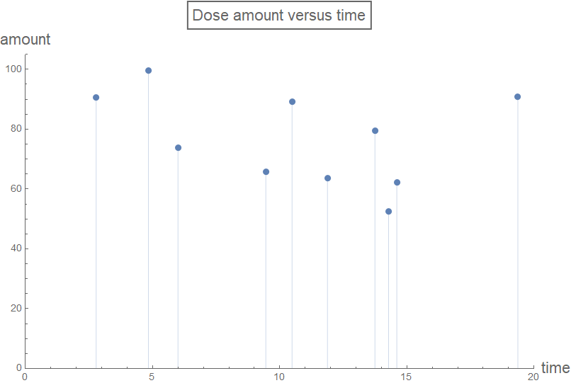
A random list "testDataList" of dose schedule and amount: {{time1, amount1}, {time2, amount2}, {time3, amount3},... } was generated to illustrate the case of random drug dosing amounts and intervals (the list is sorted from smallest to largest by time/schedule - in order to be interpreted correctly by the function rxnGeneral). This random dose schedule-amount regime is visualized below.
testDataList =
  Sort[Table[{RandomReal[{0, 20}], RandomReal[{50, 100}]}, {k, 1,
     10}], #1[[1]] < #2[[1]] &];
maxDose = Max[testDataList[[All, 2]]];

plotLabel1 = Style[Framed["Dose amount versus time"], 16];
axesLabel1 = {Style["time", 16], Style["amount", 16]};
plotRange = {{0, 20}, {0, Automatic}};
listPlot =
 ListPlot[testDataList, Filling -> Axis, PlotRange -> plotRange,
  PlotLabel -> plotLabel1, AxesLabel -> axesLabel1,
  ImageSize -> Large]
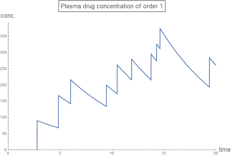
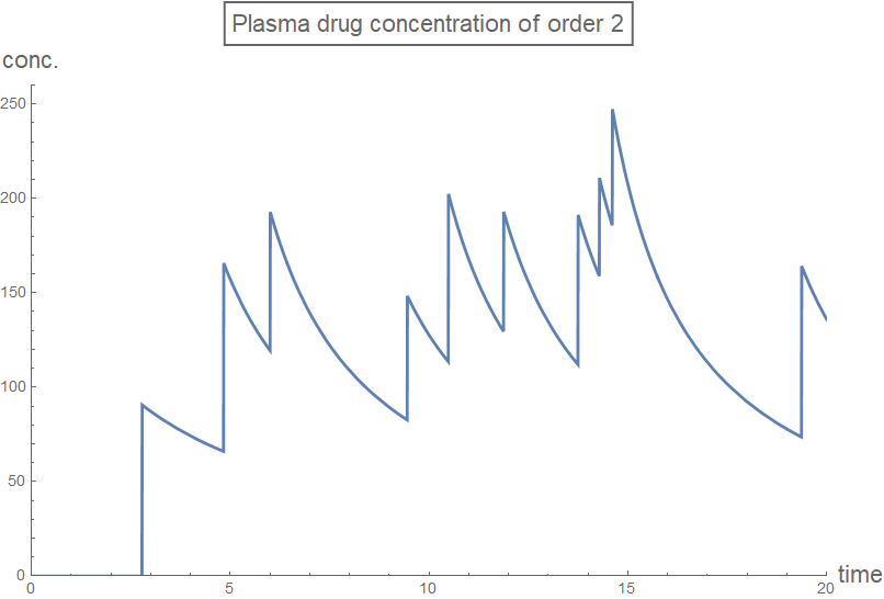
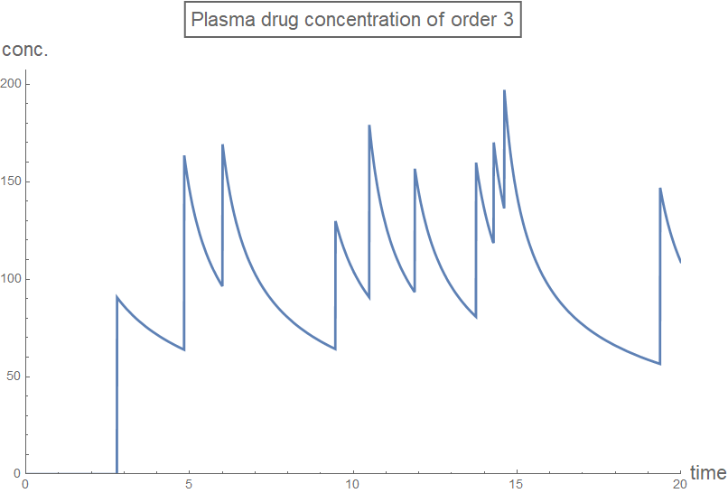
The reaction rate of these simulated drug(s) is chosen so that the maximum dose would reduce to half in five units of time (the reaction rate is tabulated in list sol2).
Off[Solve::ifun];
Off[DSolveValue::bvnul];

sol = DSolveValue[{y'[x] == -r y[x]^n, y[0] == A}, y[x], x];
sol1 = Values[Solve[(sol //. {x -> 5}) == A/2, r]][[1, 1]];
sol2 = Insert[sol1 //. {A -> maxDose, n -> {0, 2, 3}}, Log[2]/5, 2];


axesLabel2 = {Style["time", 16], Style["conc.", 16]};
Column[Table[
  plot[n] =
   Plot[rxnGeneral[t, testDataList, sol2[[n + 1]], n], {t, 0, 20},
    PlotRange -> plotRange,
    PlotLabel ->
     Style[Framed[
       StringJoin["Plasma drug concentration of order ",
        ToString[n]]], 16], AxesLabel -> axesLabel2,
    PlotStyle -> Thick,
    ExclusionsStyle -> {{Thick, ColorData[97, "ColorList"][[1]]},
      None}, ImageSize -> Large],
  {n, 0, 3, 1}]]
VI. Conclusion
Several computation models for plasma drug concentration were derived, which enable the visualization of medication's concentration profile during the treatment regime. Furthermore, the models - especially the two closed-form piecewise functions for the simplest and the most common types of prescription - specify certain conditions of dose amount and schedule to better prescribe pharmaceuticals.
References
Pharmacology 101 [Internet]. [updated 2011]. Anabolic Steroid Calculator; [cited 2019 June 27]. Available from: http://www.anabolicsteroidcalculator.com/pharmacology101.php
Steroid Calculator [Internet] [cited 2019 June 27]. Available from: https://steroidcalc.com/
Pollock M, Bazadua O, Dobbie A. Appropriate Prescribing of Medications: An Eight-Step Approach. Am Fam Physician. 2007; 75(2):231-236. Available from: https://www.aafp.org/afp/2007/0115/p231.html
Elimination Kinetics [Internet]. [updated 2009 July]. Université de Lausanne; [cited 2019 June 27]. Available from: https://sepia2.unil.ch/pharmacology/index.php?id=94
Borowy C, Ashurst J. Physiology, Zero and First Order Kinetics [Internet].[updated 2019 February 02]. Treasure Island, FL: StatPearls Publishing LLC; 2019; [cited 2019 June 27]. Available from https://www.ncbi.nlm.nih.gov/books/NBK499866/
Kinetics and Pharmacokinetics Introduction [Internet]. [updated 2017]. A Kibbe. Wilkes University; [cited 2019 June 27]. Available from: http://web.wilkes.edu/arthur.kibbe/pkfive.htm


