Goal of the Project
Analyze and study algorithms for predicting if topography is land or ocean by using simple image processing to find the differences between on-land relief plots and underwater relief plots because there is a difference between simple image processing and machine learning on images
What is Topography?
Topography is a broad term used to describe the detailed study of the earth's surface. This includes changes in the surface such as mountains and valleys as well as features such as rivers and roads. It can also include the surface of other planets, the moon, asteroids, and meteors. Topography is closely linked to the practice of surveying, which is the practice of determining and recording the position of points in relation to one another. For example, this is a topography of a random place.
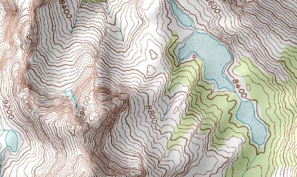
Collecting Data
Mathematica provides lots of data of various places over the world, so I take advantages of this to scrap data of on-land and underwater features for my topographies training set. The training data set includes:
200 On-land features such as capital cities, cities, buildings, mountains.
buildings = EntityList["Building"]
buildings = Take[buildings, -50]
mountains = MountainData[All]
mountains = Take[mountains, 50]
cities = EntityList["City"] // Flatten
cities = Take[cities, -50]
200 Under-water features such as trenches, basins, seamounts, etc.
underseafeatures =
 DeleteMissing[
   EntityValue[EntityClass["Ocean", "Seas"], "UnderseaFeatures"]] //
  Flatten
underseafeatureslist = Take[underseafeatures, -200]
Image Processing
I've done various approaches onto this Image Processing step but only one is suitable.
First Proposal
First, I was trying to calculate the slope of each topography by the following formula:
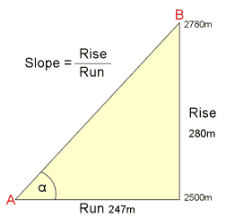
However, it will not work effectively if there are on-land topography and underwater one having the same slope. Consequently, the machine will not be able to differentiate which is land and which is ocean.
Second Proposal
Therefore, I moved on to my second proposal from my mentor Harshal, which is using Discrete Fourier Transformation to convert an image into a matrix. As I can see, the transformedimages using DFT do not help much because I can not distinguish the differences between images although the right one is land and the left one is ocean
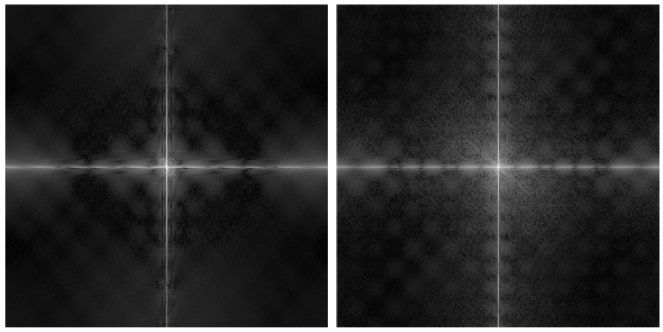
As I can see, the transformed images using DFT do not help much because I can not distinguish the differences between images although the right one is land and the left one is ocean.
Third Proposal
Finally, my final solution is applying a high-frequency filter on the images. High frequency filtered output was easy to distinguish since surface above water is generally rough when compared to the surface underwater.
Initially, start with 2 relief plots, one is the plot of Mount Everest and one is the plot of Mariana Trench.
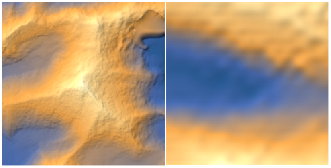
From this point, I can clearly see that the left one is Everest and the right one is Mariana Trench. The reason I can differentiate those two images because the image on the right side is rough, which means it has a high probability to be land and the image on the left side is smooth, which implies that it has a high probability to be ocean. So, let's try to find out a way to programmatically figure out these differences!
capitalcitieselevationPlots =
 ReliefPlot[
    Reverse[GeoElevationData[#, GeoRange -> Quantity[4, "Kilometers"],
       GeoProjection -> Automatic]], ImageSize -> Medium,
    ColorFunction -> GrayLevel, Frame -> False,
    PlotRangePadding -> None] & /@ capitalcities
buildingselevationPlots =
 ReliefPlot[
    Reverse[GeoElevationData[#, GeoRange -> Quantity[4, "Kilometers"],
       GeoProjection -> Automatic]], ImageSize -> Medium,
    ColorFunction -> GrayLevel, Frame -> False,
    PlotRangePadding -> None] & /@ buildings
mountainselevationPlots =
 ReliefPlot[
    Reverse[GeoElevationData[#, GeoRange -> Quantity[4, "Kilometers"],
       GeoProjection -> Automatic]], ImageSize -> Medium,
    ColorFunction -> GrayLevel, Frame -> False,
    PlotRangePadding -> None] & /@ mountains
citieselevationPlots =
 ReliefPlot[
    Reverse[GeoElevationData[#, GeoRange -> Quantity[4, "Kilometers"],
       GeoProjection -> Automatic]], ImageSize -> Medium,
    ColorFunction -> GrayLevel, Frame -> False,
    PlotRangePadding -> None] & /@ cities
underseafeatureselevationPlots =
 ReliefPlot[
    Reverse[GeoElevationData[#, GeoRange -> Quantity[4, "Kilometers"],
       GeoProjection -> Automatic]], ImageSize -> Medium,
    ColorFunction -> GrayLevel, Frame -> False,
    PlotRangePadding -> None] & /@ underseafeatureslist
Those lines of code above transfer all the locations we got into the relief plots.
In the next step, I am going to apply a high-frequency filter on the images. To illustrate, for each relief plot, I turned in into black and white and also made the black and white version blurred then found the differences between those two and thus dilate it. This is how I did it in code.
finalcapitalcitieslist =
 Dilation[ImageDifference[Blur[#, 20], #], 10] & /@
  capitalcitieselevationPlots
finalbuildingslist =
 Dilation[ImageDifference[Blur[#, 20], #], 10] & /@
  buildingselevationPlots
finalmountainslist =
 Dilation[ImageDifference[Blur[#, 20], #], 10] & /@
  mountainselevationPlots
finalcitieslist =
 Dilation[ImageDifference[Blur[#, 20], #], 10] & /@
  citieselevationPlots
finalunderseafeatureslist =
 Dilation[ImageDifference[Blur[#, 20], #], 10] & /@
  underseafeatureselevationPlots
This returns:
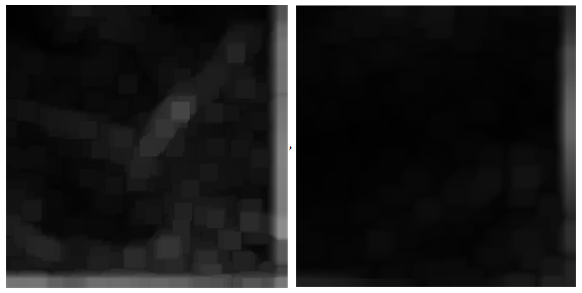
These are two images are the images of Mount Everest and Mariana Trench after applying the high-frequency filter. As mentioned above, the left one is Mount Everest and the right one is Mariana Trench. Henceforth, the differences are lots of "bubbles" in the left image compare to the right one where the "bubbles" represent the abrupt changes in the initial topography.
Creating Training Set
I gathered all the separated training sets (capital cities, cities, buildings, mountains, undersea features) into a larger training set.
finalonlandlist =
 Join[finalcapitalcitieslist, finalcitieslist, finalbuildingslist,
  finalmountainslist]
finalunderseafeatureslist = finalunderseafeatureslist
finaltraininglist = Join[finalonlandlist, finalunderseafeatureslist]
Generating Classify Function
Creating the classify function base on the training set and also the result of each element in the set and the machine got the best fit line for my model by applying Logistic Regression method.
landExamplesAndClasses = (# -> "Land" &) /@ finalonlandlist;
seaExamplesAndClasses = (# -> "Sea" &) /@ finalunderseafeatureslist;
predict =
 Classify[Union[landExamplesAndClasses, seaExamplesAndClasses]]
Creating the Final Function to Return Probabilities
I created the final function which returns the probabilities of both land and sea as the input is a topography of an arbitrary area.
predictor[img_] :=
 predict[Dilation[ImageDifference[Blur[img, 20], img], 10],
   "Probabilities"] // Normal
test = ReliefPlot[topography, Frame -> False, PlotRangePadding -> None]
predictor[test]
An Application: "Generating Temperature Map and Smooth Plot"
In this extra challenge, I randomly chose a place and generate the heat map of it and the smooth map as well.
Generating Temperature Map
What I have done was followed by this list:
- Get the coordinates of the current location.
- From current location, move to its right 15 times for 8000 meters in each step to get a list of new coordinates.
- From each coordinate in the list above, move downwards 15 times for 8000 meters in each step to get a list of new coordinates.
- Rearrange the list of coordinates vertical instead of horizontal.
- Join the lists of coordinates above all together into a big list.
- Make a list of plots for each coordinate in the list above.
- For each plot, apply the Final Function the get the Probability of Land and Water.
- Collect all the Land Probability of each plot and Arrange them into a 16x16-sized matrix.
From the 16x16-sized matrix, convert each number into Thermometer Colors ranging from - 0,5 to 0.5.
vitri = GeoPosition[Here]
vitringang =
 Table[GeoDestination[GeoPosition[vitri], {dist, 90}], {dist, 0,
   120000, 8000}]
vitridoc =
 Table[GeoDestination[GeoPosition[#], {dist, 180}], {dist, 8000,
     120000, 8000}] & /@ vitringang
vitridocdachinhsua = Table[vitridoc[[All, n]], {n, 1, 15}]
tatcavitri = Join[vitridocdachinhsua, vitringang] // Flatten
bando = ReliefPlot[
    Reverse[GeoElevationData[{#, {(# /. GeoPosition[x_] -> x)[[1]] -
         0.05, (# /. GeoPosition[x_] -> x)[[2]] + 0.05}},
      GeoRange -> Quantity[4, "Kilometers"],
      GeoProjection -> Automatic, GeoCenter -> Automatic]],
    ImageSize -> Medium, ColorFunction -> GrayLevel, Frame -> False,
    PlotRangePadding -> None] & /@ (GeoPosition /@ tatcavitri)
topo1 = predictor[#] & /@ bando // Flatten
bandomoi =
 Partition[
  Values[topo1][[#]] & /@ Flatten[Position[Keys[topo1], "Land"]], 16]
MatrixPlot[bandomoi - .5,
 ColorFunction -> ColorData["ThermometerColors"]]
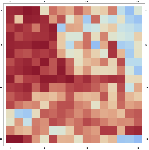
And it returns:
Let's compare it to the actual map:
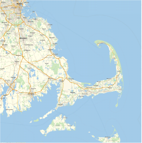
The temperature map approximately matches the actual map. However, at some points, for instance, in the sea, the color of the pixel is more red than blue. I tried to figure out the reason and found out that it might be rough because it became a water body only recently approximately couple of tens of thousands of years ago.
Generating Smooth Plot
To do this, I just applied quite same process as generating the Temperature Map above.
point1 = GeoPosition[{11.111457, 107.636774}]
point2 = GeoPosition[{11.111457, 109.803591}]
point3 = GeoPosition[{8.991341, 107.636774}]
point4 = GeoPosition[{8.991341, 109.803591}]
rong = UnitConvert[GeoDistance[point1, point2], \!\(\*
NamespaceBox["LinguisticAssistant",
DynamicModuleBox[{Typeset`query$$ = "meters", Typeset`boxes$$ =
       TemplateBox[{
InterpretationBox[" ", 1], "\"m\"", "meters", "\"Meters\""},
        "Quantity", SyntaxForm -> Mod],
       Typeset`allassumptions$$ = {{
        "type" -> "Clash", "word" -> "meters",
         "template" -> "Assuming \"${word}\" is ${desc1}. Use as \
${desc2} instead", "count" -> "2",
         "Values" -> {{
           "name" -> "Unit", "desc" -> "a unit",
            "input" -> "*C.meters-_*Unit-"}, {
           "name" -> "Word", "desc" -> "a word",
            "input" -> "*C.meters-_*Word-"}}}},
       Typeset`assumptions$$ = {}, Typeset`open$$ = {1, 2},
       Typeset`querystate$$ = {
       "Online" -> True, "Allowed" -> True,
        "mparse.jsp" -> 0.3739998`7.0244163634533505,
        "Messages" -> {}}},
DynamicBox[ToBoxes[
AlphaIntegration`LinguisticAssistantBoxes["", 4, Automatic,
Dynamic[Typeset`query$$],
Dynamic[Typeset`boxes$$],
Dynamic[Typeset`allassumptions$$],
Dynamic[Typeset`assumptions$$],
Dynamic[Typeset`open$$],
Dynamic[Typeset`querystate$$]], StandardForm],
ImageSizeCache->{80., {8., 18.}},
TrackedSymbols:>{
         Typeset`query$$, Typeset`boxes$$, Typeset`allassumptions$$,
          Typeset`assumptions$$, Typeset`open$$,
          Typeset`querystate$$}],
DynamicModuleValues:>{},
UndoTrackedVariables:>{Typeset`open$$}],
BaseStyle->{"Deploy"},
DeleteWithContents->True,
Editable->False,
SelectWithContents->True]\)] // QuantityMagnitude
dai = UnitConvert[GeoDistance[point1, point3], \!\(\*
NamespaceBox["LinguisticAssistant",
DynamicModuleBox[{Typeset`query$$ = "meters", Typeset`boxes$$ =
       TemplateBox[{
InterpretationBox[" ", 1], "\"m\"", "meters", "\"Meters\""},
        "Quantity", SyntaxForm -> Mod],
       Typeset`allassumptions$$ = {{
        "type" -> "Clash", "word" -> "meters",
         "template" -> "Assuming \"${word}\" is ${desc1}. Use as \
${desc2} instead", "count" -> "2",
         "Values" -> {{
           "name" -> "Unit", "desc" -> "a unit",
            "input" -> "*C.meters-_*Unit-"}, {
           "name" -> "Word", "desc" -> "a word",
            "input" -> "*C.meters-_*Word-"}}}},
       Typeset`assumptions$$ = {}, Typeset`open$$ = {1, 2},
       Typeset`querystate$$ = {
       "Online" -> True, "Allowed" -> True,
        "mparse.jsp" -> 0.3739998`7.0244163634533505,
        "Messages" -> {}}},
DynamicBox[ToBoxes[
AlphaIntegration`LinguisticAssistantBoxes["", 4, Automatic,
Dynamic[Typeset`query$$],
Dynamic[Typeset`boxes$$],
Dynamic[Typeset`allassumptions$$],
Dynamic[Typeset`assumptions$$],
Dynamic[Typeset`open$$],
Dynamic[Typeset`querystate$$]], StandardForm],
ImageSizeCache->{80., {8., 18.}},
TrackedSymbols:>{
         Typeset`query$$, Typeset`boxes$$, Typeset`allassumptions$$,
          Typeset`assumptions$$, Typeset`open$$,
          Typeset`querystate$$}],
DynamicModuleValues:>{},
UndoTrackedVariables:>{Typeset`open$$}],
BaseStyle->{"Deploy"},
DeleteWithContents->True,
Editable->False,
SelectWithContents->True]\)] // QuantityMagnitude
soluongbuocnhayngang = rong/8000 + 1 // Floor
soluongbuocnhaydoc = (dai - 8000)/8000 + 1 // Floor
vitringang1 =
 Table[GeoDestination[GeoPosition[point1], {dist, 90}], {dist, 0,
   rong, 8000}]
vitridoc1 =
 Table[GeoDestination[GeoPosition[#], {dist, 180}], {dist, 8000, dai,
     8000}] & /@ vitringang1
vitridoc1dachinhsua =
 Table[vitridoc1[[All, n]], {n, 1, soluongbuocnhaydoc}]
vitridoc1dachinhsua =
 Table[vitridoc1[[All, n]], {n, 1, soluongbuocnhaydoc}]
tatcavitri1 = Join[vitridoc1dachinhsua, vitringang1] // Flatten
bando1 = ReliefPlot[
    Reverse[GeoElevationData[{#, {(# /. GeoPosition[x_] -> x)[[1]] -
         0.05, (# /. GeoPosition[x_] -> x)[[2]] + 0.05}},
      GeoRange -> Quantity[4, "Kilometers"],
      GeoProjection -> Automatic, GeoCenter -> Automatic]],
    ImageSize -> Medium, ColorFunction -> GrayLevel, Frame -> False,
    PlotRangePadding -> None] & /@ (GeoPosition /@ tatcavitri1)
topo11 = predictor[#] & /@ bando1 // Flatten
bandomoi1 =
 Partition[
   Values[topo11][[#]] & /@ Flatten[Position[Keys[topo11], "Land"]],
   soluongbuocnhayngang] // Flatten
kethopvitrichiso = MapThread[Rule, {tatcavitri1, bandomoi1}]
GeoSmoothHistogram[kethopvitrichiso,
 ColorFunction -> ColorData["ThermometerColors"]]
And here it is, this is the Smooth Map of a part of Vietnam which contains sea and land.
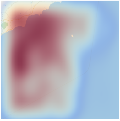
Red regions in the heat map show land and blue show ocean and as visible
Wrapping-up
To summarize, in the first step, I collected the topographies from both on-land and underwater. Then in the second one, the most complicated step, I had tried to use Discrete Fourier Transform (DFT) for a topography image into the matrix, but the problem was that all Fourier images were very similar. Then I tried applying a high-frequency filter on the images. High frequency filtered output was easy to distinguish since surface above water is generally rough when compared to the surface underwater. After the Image Processing Step, I created the two set of training sets, one is on-land training set and another one is underwater features training set. Hence, I went straight to build the classify function and the Final Function to Return Probabilities of "Land" and "Sea" as well. Finally, for an extra challenge also a nice application in other words for my project, I generated a Temperature Map of a part of Boston and tried to compare it to the actual map and the generated heat map is similar to the real map.
Future Works
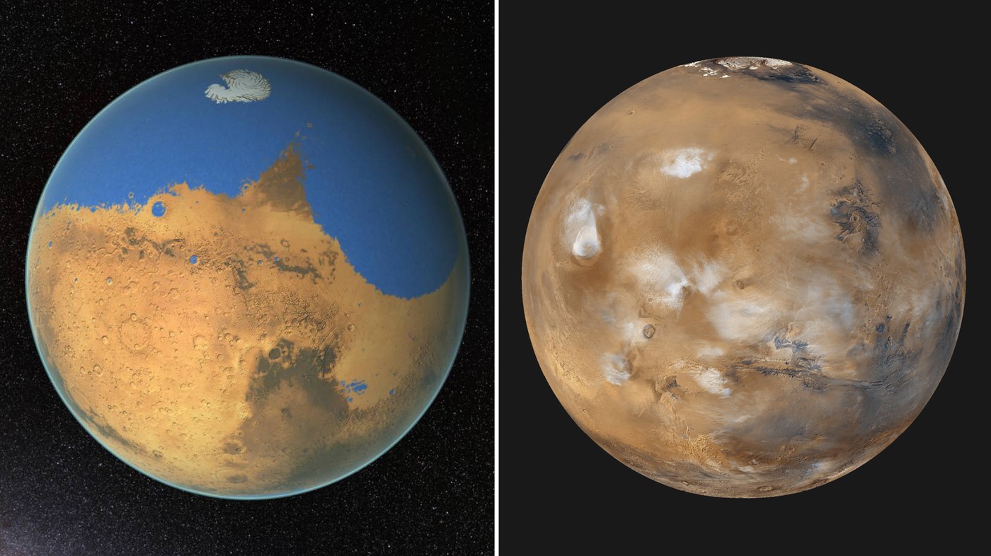
As we can see, from an arbitrary relief plot of a location, it is possible to turn the relief one into the thermometer surface where blue represents "Sea" and red represents "Land" by using the probabilities that the classifier returned. The first thing that needs to be done is to think of other crucial parameters that can be used, like water bodies around buildings, etc. to increase the accuracy. After increasing the accuracy and interesting thing to do would be to analyze the topography of other celestial bodies (like Mars) and then predict regions where liquids flowed on the surface.
Are these the images of wet Mars in the past and current Mars? Who knows.
Special Thanks
I would like to give my special thanks to my mentor Mr. Harshal Gajjar for guiding me and also Mr. Mads Bahrami for giving me more challenges!
Final Project GitHub link