Introduction

Over the past few years, there's been an unprecedented amount of excitement surrounding the idea of artificial intelligence and neural networks as catch-all solutions to any and all big-data problems. In today's world, a data scientist's toolbox is incomplete without a variety of RNNs, LSTMs, GANs, and whatever other initialisms will best catch the eye of CEOs looking to "steer their company into the future". These tools are powerful and often practical, but AI's uninhibited usage has grown to the point that the terms "deep learning" and "AI" have been become buzzwords typifying the blind overconfidence of modern business technology. Many criticize deep learning for its opacity, with a mechanism incomprehensible to humans - just an incredibly long, high-dimensional matrix of weights with no tangible significance. This lack of human understanding, and therefore human correction, begs the question: are neural networks fallible? And even more pressing: are they vulnerable?

Abstract

This project implements a framework for generating adversarial examples: input data crafted to cause a neural network to produce unexpected, or targeted incorrect behavior. Such a problem is split into two tasks: generating what should be easily-classifiable inputs that fool the neural network, and generating random-looking inputs that return targeted, high-probability results when fed to the neural network. We implement the Fast Gradient Sign Method (Goodfellow 2014b) for the former, and an original algorithm modeled after FGSM for the latter. Using these algorithms, we examine whether these adversarial examples are in fact edge cases, or make up a majority of the neural network's classification space. We also construct two models to minimize the effect of adversarial examples, and evaluate their accuracy at detecting and overcoming adversarial images on the MNIST database. We also provide a general purpose function to adversarially attack an arbitrary neural network for public use in the Wolfram Function Repository.

Creation

The first type of adversarial example we generate are "perturbed" adversarial examples, where the smallest possible change is made to the image to throw off the results of the neural network. We implement the Fast Gradient Sign Method (FGSM). This is an algorithm originally described by Goodfellow (2014) that makes the smallest possible change to an image to maximize the loss function of the neural network. It does this by calculating the sign of the gradient of the loss function with respect to the input. What this gives is effectively an image representing how much changing each RGB value in the image affects the returned probability overall, which is then interpreted to produce an image that minimizes that probability, and maximizes loss. The following is a function for calculating FGSM in Mathematica:

imageAdversarialPerturbed[sourceImg_,net_,epsilon_]:= With[{
    lossNet=NetChain[{
       NetReplacePart[net,{"Output" -> None}], 
       AggregationLayer[Max,1], 
       ElementwiseLayer[-Log[#]&]
    }],
    encoder=NetExtract[net,"Input"]
},
ImageResize[NetDecoder[encoder][encoder[sourceImg]+epsilon*Sign[lossNet[sourceImg,NetPortGradient["Input"]]]],ImageDimensions@sourceImg]]

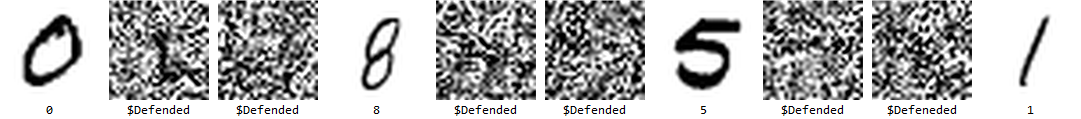
Using this function, we can make images that humans can easily identify that the neural network fails to recognize:

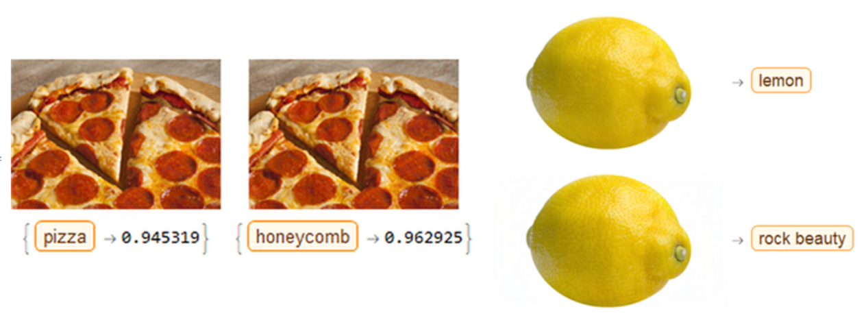
But we can also generate examples targeted towards a certain class of the neural network, maximizing a specific probability rather than minimizing them all. This is done by somewhat reversing the process of FGSM, with respect to a slightly different neural network. A loss function is usually calculated by somehow comparing the output and the expected output: but for targeted adversarial attacks, we can define a new loss function where we "fake" the expected output such that it is probability 1 for whatever class we decide, and 0 for all others. Then, we perform gradient descent, not on the weights of the network, but on the input pixels of the image, using this "fake loss" function to see how each pixel effects the probability of the class we want. With very small step size, repeating this process guarantees an optimal path to the 'nearest' image with high-confidence for a class of our choosing. Here is this algorithm implemented in Mathematica:

ClearAll[imageAdversarialTargeted]
Options[imageAdversarialTargeted] = {"Epsilon" -> 0.01, "MaxSteps" -> 15, 
   "IncreaseConfidence" -> True};
imageAdversarialTargeted[net_, sourceImg_Image, maxClass_: None, 
  OptionsPattern[]] := With[{
        lossNet = NetChain[{
             NetReplacePart[net, {"Output" -> None}],
             If[maxClass === None,
                 AggregationLayer[Max, 1],
                 PartLayer[maxClass]
                 ],
             ElementwiseLayer[-Log[#] &]
         }],
        encoder = NetExtract[net, "Input"]
    },
  ImageResize[
   Nest[NetDecoder[encoder][
      encoder[#] - 
       If[OptionValue["IncreaseConfidence"], 1, -1]*
        OptionValue["Epsilon"]*
        Sign[lossNet[#, NetPortGradient["Input"]]]] &, sourceImg, 
    OptionValue["MaxSteps"]], ImageDimensions@sourceImg]]

This can give us some truly cool images:

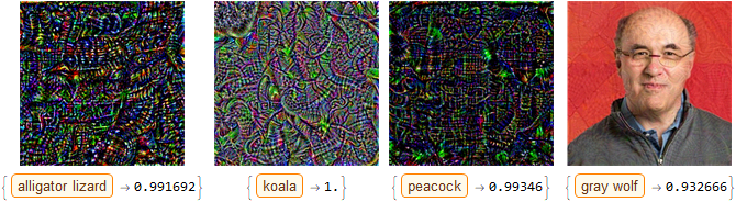
Check out the microsite I put together that takes a number 1-1000 representing a class, and gives you an image with high-probability for that class!

Calculation

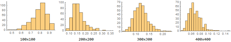
The next part of my project involved statistical analysis of these adversarial examples. Sampling randomly from the space of all images of different sizes, we can plot a histogram of the average highest probability when a random image is put through our image identification net:

But how many of these are real examples and how many adversarial? Well, we can randomly sample from the space of images which the neural network classifies with high confidence by using our algorithm above on random images, and use a second neural network with a different architecture to "verify" the classification of our first. If they are somewhat in agreement, it is probably a real image. If this disparity is very large, it is almost certainly adversarial. For example, if our victim network classifies an image as 100% a pineapple, and our verifier net classifies it as 2% a pineapple, we can be sure that the inputted image is adversarial to our victim net, rather than an actual example of a pineapple.

im2 = NetModel["Wolfram ImageIdentify Net V1"]
generateAdversarial[size_] := 
 imageAdversarialTargeted[imageIdentify, RandomImage[1, size, ColorSpace -> "RGB"], 
None,"MaxSteps"->3]
  advReal[size_, sample_] := 
 Table[
   With[{a = generateAdversarial[size]}, 
    imageIdentify[a, "TopProbabilities"][[1]][[2]] - 
     im2[a, "TopProbabilities"][[1]][[2]]], {n, 1, sample}]
     Histogram@advVsreal
prob = FindDistribution[advVsreal];
Probability[x < 0.1, x \[Distributed] prob]

Here is the histogram of the difference between the two network's confidence for random images:

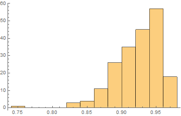
If the difference between these two network's confidence is above $.9$, we can be sure that the image is adversarial. Extrapolating probability from the histogram above, we find that the probability that a given high-confidence image is actually real and not adversarial is $1$ in $1.70154\times 10^{34}$ - in other words, negligible.

I also found that these adversarial examples are much more "robust" than normal images, and even more robust than training images. I implemented the inverse of my targeted-adversarial algorithm to travel away from high probabilities as quickly as possible, and found that adversarial examples take, on average, 5 times as many steps as training images.

Counteraction

I also implemented two methods to minimize adversarial examples, one well-known and the other original. The first is simple direct adversarial training - using the above algorithms to generate tons of adversarial examples as training data, and training a new neural network with the same architecture as the first to classify examples as "adversarial" or "not adversarial". I used a toy example with MNIST and the standard classifier network for MNIST known as "lenet", but the idea scales to any neural network with a good enough GPU. Whereas machine learning that takes user input and gives the user output is vulnerable due to the ability to optimize inputs for a given output, this filter can act completely server-side and therefore not be accessible by the user. An implementation of this method was shown to be very close to 100% effective, correctly filtering 998 out of 1000 randomly generated examples.

The second method is an original algorithm I have nicknamed the "democratic probabilistic reasoning kernel", or "DPRK" for short. DPRK uses a collection of neural networks trained on the same architecture but initialized differently and averages their softmax layers to get the final probability vector. It takes advantage of a mysterious property of adversarial examples for different neural networks with similar architecture: they are transferable, but give different results. This means that high-confidence adversarial examples for one neural network give high-confidence results for another neural network, but it will be high-confidence for a different class.

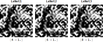
I was able to theorize a reason for this mechanism, based on the statistics presented above. For more information, check out my computational essay! When the architectures are exactly the same, this phenomenon stretches to the extreme - moving the gradient of one neural network in the direction of a class C moves the gradient of another neural network in the direction of class D by the exact same magnitude. The result of this is that adversarial examples get "stuck" between neural networks. When it tries to optimize the gradient of one, it de-optimizes the gradient of another. The best, therefore, that the neural network can do is to split probabilities evenly between the neural network: so if we have 5 neural networks, it will give a probability vector containing, among your classes, 5 elements with 0.2 probability. The more neural networks you add, the more this probability goes down. The more classes you have, the more this probability goes down. This method was able to stop 100% of attacks on MNIST, with an actual increase in accuracy on the normal test set.

Conclusion and Implications

The results of this project can only be described as "bittersweet". It turns out that adversarial examples are not only directly instantiable but also make up a majority of the space of images classified by any given network as high-probability. Neural networks are therefore incredibly vulnerable to targeted attacks of this manner, especially those dealing with low-dimensional vectors. Theoretically, although not implemented here due to deficiencies in Mathematica's machine learning library, this adversarial method works for any neural network on which you can perform backpropagation. Furthermore, there is no need to actually have access to the internals of the neural network, just the input and output.

And yet there is some hope. The transfer of adversarial examples between neural networks with arbitrary labeling can be exploited to filter out, theoretically, all adversarial examples, something that has never been accomplished before. In practical settings, it was also shown that just 2 neural networks, the original and a 'filter network', is sufficient to filter out most, if not all adversarial examples.

Yet one may consider these solutions, even if efficient, to be "band-aids" on fundamental flaws in the architecture of neural networks. Here, it is an interesting question to study the difference between ANNs and actual neural circuits in the context of this project. Humans experience the phenomena of "optical illusions", but the way we experience these illusions reveals an important difference between machine intelligence and conscious intelligence: the ability to understand when you are being fooled. This "consciousness of consciousness" is higher-order than simple self-consciousness, as it requires not only awareness of your own consciousness but pattern-recognition applied to it. My project shows that the current structure of ANNs does not allow this kind of analysis, modelling only "first-order-thinking". One could create another neural network to analyze the first, but then you've just shifted (and arguably augmented) the fundamental problem. It is only when you have an architecture that models itself, that it can begin to undergo learning in a non-trivial manner, achieving the type of cognitive accuracy that humans do. A mathematical description of such an architecture would, hopefully, allow theoretically for AGI while circumventing the question of actually defining consciousness.