Implementing a Visualizer for DNA Sequence Alignments
Introduction
In the field of bioinformatics, DNA sequence alignment is a method of arranging sequences to find similarities between them. These similarities may be caused by similar function, structure, or evolutionary origin. These alignments are generated by computer algorithms. There are two types, pairwise alignment and multi-sequence alignment. For this project, I only used pairwise alignment. The two types of pairwise alignment are global alignment and local alignment developed by Needleman/Wunsch and Smith/Waterman respectively. Global alignment attempts to align the sequences along the entire input, while local alignment aligns within a fixed distance from the current character. My goal was to create a visual output that represents sequence alignment.
Abstract
This project creates a visualization function that takes an input of a reference DNA sequence and multiple comparison sequences and outputs several different visual models that show the similarities and differences between them. It utilizes the functions, SequenceAlignment, LongestCommonSubsequence, NeedlemanWunschSimilarity, and SmithWatermanSimilarity, which are built-in functions of the WolframLanguage that use the classic algorithms for sequence alignment as created by the researchers Needleman, Wunsch , Smith, and Waterman. The result will yield figures and graphs to show the alignment . This tool can be used to study evolutionary origins of species, detect mutations, and analyze other biological relationships.
Creating the Visualization
Alignment Visualizer
My initial goal was to create an alignment visualizer similar to the commercial sequence alignment visualizations. This entailed lining up the similar bases in columns that are easily differentiated, and showing the bases that differ as well. This meant it would be necessary to insert spaces when bases were present in one strand and absent in the other. I researched the different types of alignment, and I decided to start with pairwise alignment and possibly expand towards multi-sequence alignment.
My first thought was to begin developing an algorithm to align the sequences, but I realized, to my delight, that there were various built-in tools that help with biological computation including the functions SequenceAlignment, LongestCommonSubsequence, NeedlemanWunschSimilarity, and SmithWatermanSimilarity.
I started playing around with the SequenceAlignment results, and tried to make the visualizer with the lined-up columns. This proved to be difficult task. After some research, I discovered a Wolfram Demonstration that used the alignment function to align English dictionary words. Its formatting structure proved to be helpful, and I was able to format the SequenceAlignment results as desired. I also added a color association to color the letters A,T,G,C in different colors. This is how it works:
Below, I removed spaces and line breaks and format into a framed row:
picture[d_String, e_String] :=
 Text@Row[Flatten@(Map[format,
      SequenceAlignment[
       StringDelete[ToUpperCase[d], " " | "\n" | "\t"],
       StringDelete[ToUpperCase[e], " " | "\n" | "\t"],
       MergeDifferences -> False]]), Frame -> True]
I formatted each term of the output of Sequence Alignment and assigned coloring for matches, substitutions, insertions, deletions:
format[{a_String, b_String}] :=
  Column[{colored[a], colored[b]}, Spacings -> 1,
   Background -> Blend[{LightRed, White}, .17]];
format[{a_String, ""}] :=
  Column[{colored[a], StringJoin@Table["-", {StringLength[a]}]},
   Spacings -> 1, Background -> Blend[{LightRed, Red}, .12]];
format[{"", b_String}] :=
  Column[{StringJoin@Table["-", {StringLength[b]}], colored[b]},
   Spacings -> 1, Background -> Blend[{LightRed, Red}, .12]];
format[c_String] :=
  If[StringLength[c] > 20, format2 /@ StringPartition[c, 10], format2[c]];
format2[c_String] :=
  Column[{colored[c], colored[c]}, Spacings -> 1, Background -> LightGreen];
Next, I added color to the sequence code and made the text bold:
colored[h_String] := Row@(colorassoc /@ Characters[h])
colorassoc = <|"A" -> Style["A", RGBColor[1., 0.02, 0.87], Bold],
  "T" -> Style["T", Blue, Bold],
  "G" -> Style["G", RGBColor[0.15, 0.67, 1.], Bold],
  "C" -> Style["C", RGBColor[0.34, 0.34, 0.34], Bold]|>
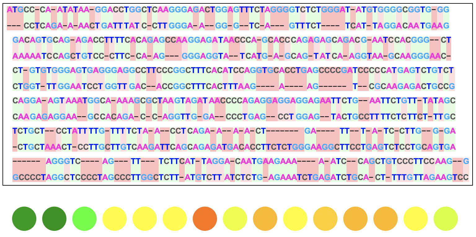
Here is the output for two DNA sequences:
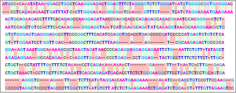
This visual displays exactly how the two sequences are aligned from the algorithm where the green, darker red, and lighter red backgrounds represent matches, deletions/insertions, and substitutions respectively.
Color Chain
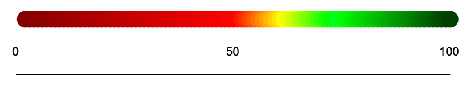
The next step was to create a visual for very long sequences- something that would be easier to look at rather than the detailed alignment visual.Some genes are only a couple hundred bases long, but most genes are thousands and thousands of bases long. I found an interesting example of alignment visualization for the human genotype compared to other primates. They used chains of colors with different percentage values to measure the percentage of difference in each 500,000 bases of the genomes. I decided to create a similar visual at a smaller scale.
For shorter sequences that are less than 10,000 bases, the sequences are analyzed in groupings of 100. For longer sequences that are more than 10,000 bases, the sequences are analyzed in groupings of 1000. One disk is generated for each chunk and is colored according to the percent similar bases it has with the reference sequence. The following scale represents the percentage of similarity and its corresponding color value:
The first step was to make the longer string the same length as the shorter string:
samelength[{a_, b_}] :=
 If[StringLength[a] >
   StringLength[b], {StringTake[a, StringLength[b]], b}, {a,
   StringTake[b, StringLength[a]]}]
Next, I calculated the number of similar bases:
basecount[{a_, b_}] :=
 If[StringLength[b] < 10000,
  samebase[First@#, #[[2]]] & /@ split[samelength[{a, b}]],
  Round /@ (Divide[#, 10] & /@ (samebase[First@#, #[[2]]] & /@
       split[samelength[{a, b}]]))]
The color chain is generated as a table of colored disks from the redgreen association:
colormap[{a_, b_}] :=
 Graphics@Table[
   Style[Disk[{n, 0},
     StringLength[a]/5000], (redgreen /@ basecount[{a, b}])[[n]]], {n,
     1, Length@(redgreen /@ basecount[{a, b}]), 1}]
This association assigns each numerical value 1-100 to a color from red to green:
redgreen =
 Join[AssociationThread[
   Range[0, 49] -> Reverse@Table[Darker[Red, n], {n, 0, .49, 0.01}]],
  AssociationThread[
   Range[50, 74] -> Table[Hue[n], {n, 0, .36, 0.015}]],
  AssociationThread[
   Range[75, 100] -> Table[Darker[Green, n], {n, 0, .75, .03}]]]
Here is an example output for two sequences:

Tables
To make the tool more useful and accessible, I decided to use a table format where multiple sequences can be compared to a single reference sequence. The first table displays all the numerical values as well as the first 30 bases and the longest common subsequence. The second table shows all of the visuals and graphs including the alignment visual and the color chain. At the bottom, the three BarCharts that show comparison between the sequences are displayed.
tables[{a_String, b_List}] :=
 Column[{table[{a, b}], table2[{a, b}],
   Row[{barall[{a, b}], gltab[{a, b}]}]}]
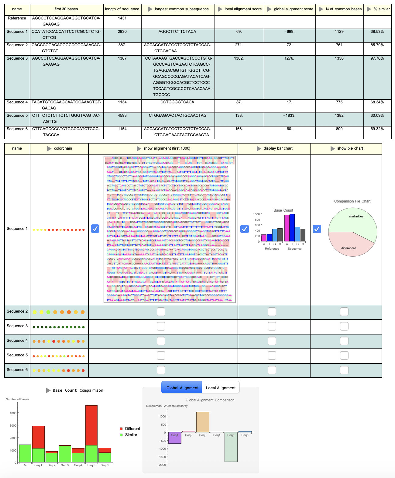
Table Features
Here are some of the other values in the first table and what they mean:
- First 30 bases: the given sequence shortened to the first thirty bases
- Length of sequence: the number of bases in the given sequence -Longest common subsequence: the longest subsequence shared by the reference and the given sequence
- Local alignment score: score given by the Smith-Waterman alignment algorithm, which aligns within a fixed distance from the current character.
- Global alignment score: score given by the Needleman-Wunsch alignment algorithm, which aligns along the other charts displayed by the tables function and what they represent:
- Number of common bases: the number of bases that are aligned between the sequences; essentially, the number of bases with a green background in the alignment figure
- Percent similarity: percent form of the number of common bases divided by the sequence length
Here are the other charts displayed by the tables function and what they represent:
- Base count BarChart: the number of each base (ATGC} counted for the reference and the given sequence
- PieChart: the number of similar bases and different bases between the first 1000 bases of the two sequences compared
- Global/local alignment BarChart: the global and local alignment scores for all of the comparison sequences
- Base count BarChart: the length of the sequences and the similar/different base ratio for the reference and all of the comparison sequences
Making it User-Friendly
Checkboxes: checkboxes were implemented to allow the user to open and minimize the visuals in the second table for easier viewing. Here is one example:
check[a_, b_] :=
 DynamicModule[{x},
  Grid[{{Checkbox[Dynamic[x]], Dynamic[If[x, picture[a, b], ""]]}}]]
OpenerView: for each one of the visuals or values that may be confusing for the user to understand an explanation that could be accessed by OpenerView. Here is one example:
colorchainopen =
  OpenerView[{"colorchain",
    "Each sequence is partitioned into sections of 100 for short \
sequences and 1000 for long sequences, and the number of aligned \
bases is counted and a colored disk is created to represent the \
percent of aligned bases given by the following scale:" \
redgreenscale}];
User Interfaces
My last task was to implement an interface that would allow the user to easily access the tool. I created two interfaces: one that takes a freeform input where the user can copy and paste their own DNA sequences for comparison and one that has imported Wolfram data for several genes that are common between different organisms . These interfaces have been attached at the bottom of this post.
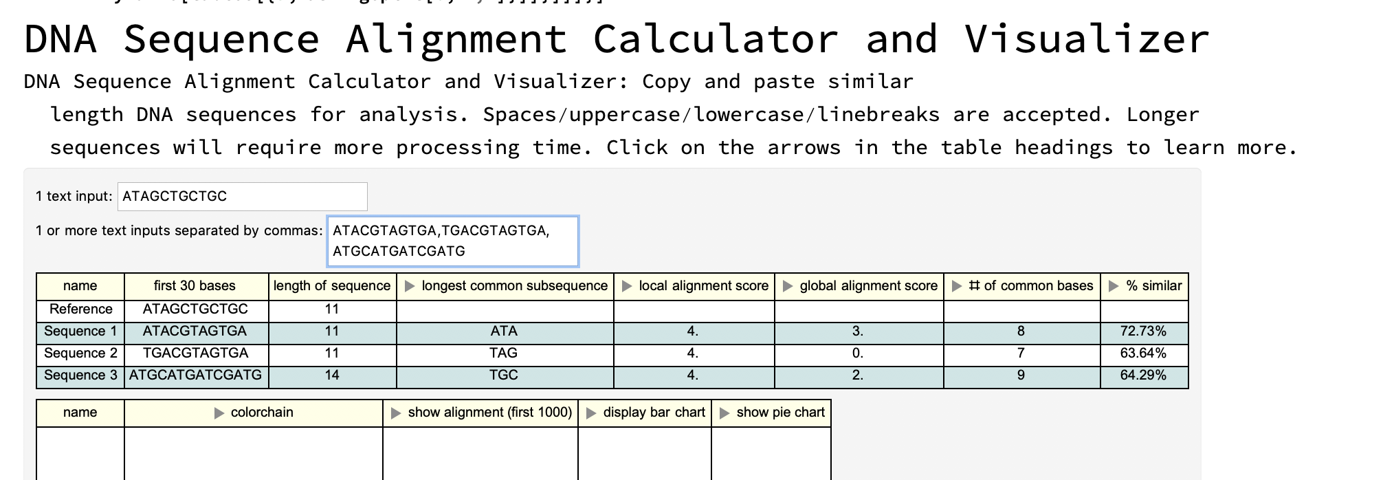
First interface: copy and paste your own DNA sequences
Column[{Style["DNA Sequence Alignment Calculator and Visualizer",
   FontSize -> 30],
  Style["DNA Sequence Alignment Calculator and Visualizer: Copy and \
paste similar length DNA sequences for analysis. \
Spaces/uppercase/lowercase/linebreaks are accepted. Longer sequences \
will require more processing time. Click on the arrows in the table \
headings to learn more. ", FontSize -> 15],
  Panel[DynamicModule[{a = "reference", b = "comparison sequences"},
    Column[{Row[{"1 text input: ", InputField[Dynamic[a], String]}],
      Row[{"1 or more text inputs separated by commas: ",
        InputField[Dynamic[b], String]}],
      Dynamic[tables[{a, StringSplit[b, ","]}]]}]]]}]
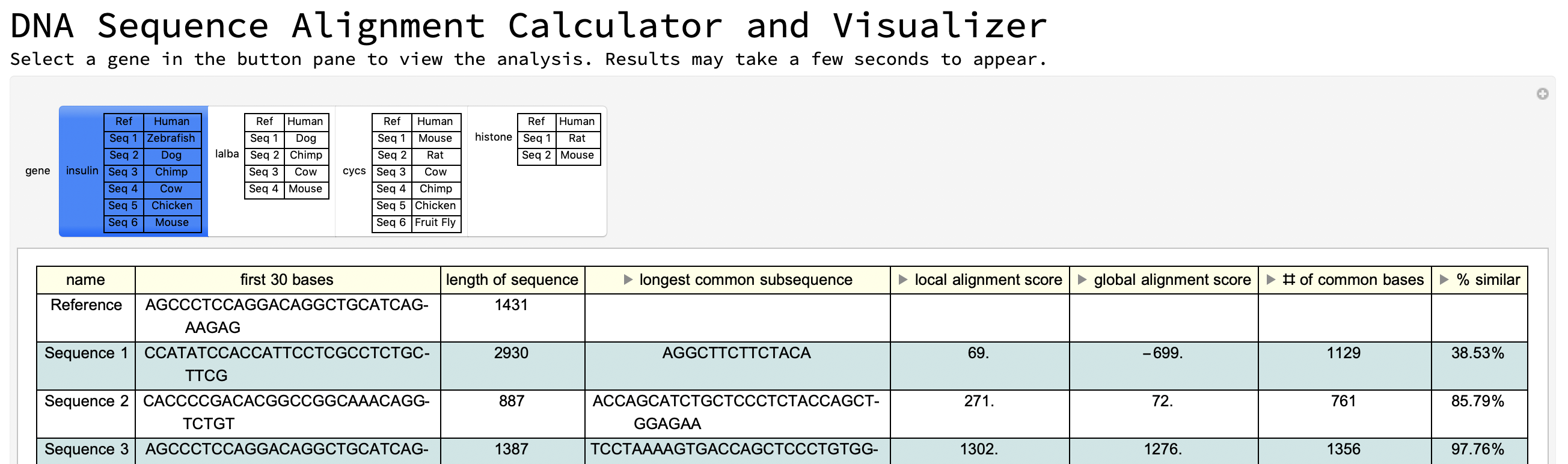
Second interface: using Wolfram Data example genes
Column[{Style["DNA Sequence Alignment Calculator and Visualizer",
   FontSize -> 30],
  Style["Select a gene in the button pane to view the analysis. \
Results may take a few seconds to appear.", FontSize -> 15],
  Manipulate[
   tables[gene], {gene, {insulin -> "insulin" grid,
     lalba -> "lalba" grid2, cycs -> "cycs" grid3,
     histone -> "histone" grid4}}, SaveDefinitions -> True]}]
Conclusion
Summary
These tools can be used to quickly analyze many sequences in reference to one sequence. Organisms that share similar bases and have similar sequence lengths and high alignment scores are more likely to have similar structure and function for that particular gene. It provides a large variety of visuals including charts and figures to compare the sequences for different purposes. It takes into account short sequence/long sequence differentiation and other syntactical differences. Possible applications include education or biological analysis.
Future
In the future, I hope to implement a DNA to mRNA codon to protein translator. This could be useful for learning about DNA transcription and translation. I could also modify the algorithm so that the sequences are compared among each other instead to a single reference strand. This would use a multiple sequence alignment algorithm instead of a pairwise sequence alignment algorithm. Another possible application would be using the results of DNA analysis to automatically generate phylogenetic trees among organisms.
Thank you to Wolfram Summer Camp for the wonderful opportunity and Lauren Cooper for being an amazing mentor!
 Attachments:


