Not because LearnDistribution is Experimental but because there aren't many details about what it actually does is why I think you should shy away from it. One can "extract" the parameters used but I don't think that all of those parameters make sense. For example one of the means is negative when you have all positive data with the leftmost of 3 "peaks" greater than zero.

data = {0.563000, 0.180000, 0.429000, 0.292000, 0.315000, 0.888000, 
   0.59100, 0.196000, 0.200000, 0.581000, 0.265000, 0.288000, 
   0.492000, 0.600000, 0.722000, 0.471000, 0.232000, 0.835000, 
   0.370000, 0.265000, 0.266000, 0.340000, 0.239000, 0.931000, 
   0.201800, 0.522000, 0.635000, 0.537000, 0.503000, 0.201000, 
   0.438000, 0.627000, 0.356000, 0.462000, 0.156000, 0.875000};

(* LearnDistribution *)
ld = LearnDistribution[data, Method -> {"GaussianMixture", "ComponentsNumber" -> 3, 
 "CovarianceType" -> "Full"}]
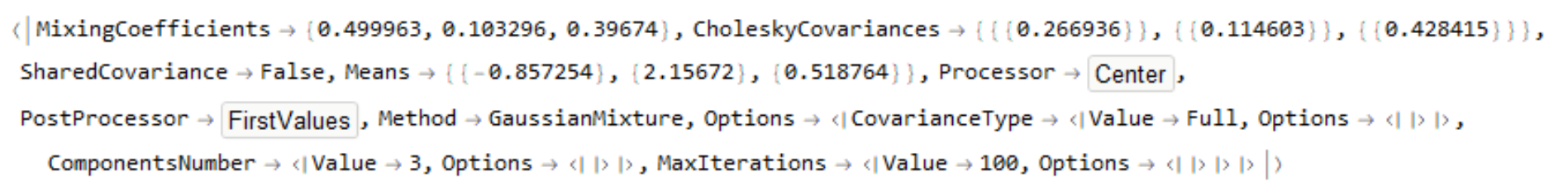
ld[[1, 6]]

I suggest fitting a mixture of Gaussian distributions in a more direct way:

(* Maximum likelihood approach *)
md = MixtureDistribution[{w1, w2, 1 - w1 - w2}, {NormalDistribution[m1, s1], 
NormalDistribution[m2, s2], NormalDistribution[m3, s3]}]
mle = FindDistributionParameters[data, md, ParameterEstimator -> "MaximumLikelihood"]

(* {w1 -> 0.467002, w2 -> 0.110224, m1 -> 0.524247, s1 -> 0.0988225, 
m2 -> 0.882558, s2 -> 0.0341755, m3 -> 0.246329, s3 -> 0.0562667} *)

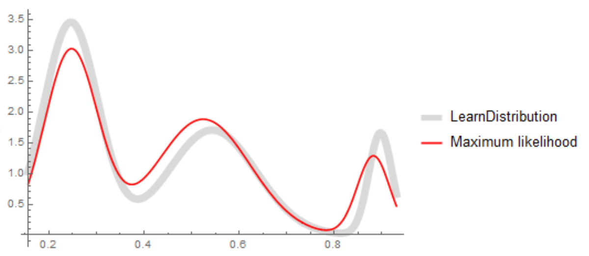
The results are not identical but at least you know how you got the maximum likelihood results:

(* Plot of results *)
Plot[{PDF[ld, x], PDF[md, x] /. mle}, {x, Min[data], Max[data]},
PlotStyle -> {{LightGray, Thickness[0.02]}, Red},
PlotLegends -> {"LearnDistribution", "Maximum likelihood"}]

Your original question is to get the estimate of the PDF. Here's that function:

PDF[md/.mle]

Function[\[FormalX], 
 1.28668 E^(-428.094 (-0.882558 + \[FormalX])^2) + 
  1.88527 E^(-51.1986 (-0.524247 + \[FormalX])^2) + 
  2.99756 E^(-157.931 (-0.246329 + \[FormalX])^2)]

Now back to your original question: How to get the parameters associated with the results from LearnDistribution? Again, I think you should avoid using LearnDistribution not because it's bad but because it's a black box with inadequate documentation. However, one can get the associated parameters at least in a reasonably precise way. We can generate a table of a bunch of values and use NonlinearModelFit because we know the variability about the curve is going to be very small.

t = Table[{x, PDF[ld, x]}, {x, Min[data], Max[data], (Max[data] - Min[data])/100}];
nlm = NonlinearModelFit[t, PDF[md, x], mle /. Rule -> List, x];
fit = nlm["BestFitParameters"]
(* {w1 -> 0.39674, w2 -> 0.103296, m1 -> 0.543333, s1 -> 0.0926299, 
 m2 -> 0.897484, s2 -> 0.0247789, m3 -> 0.245816, s3 -> 0.0577158} *)

Plot[{PDF[ld, x], PDF[md, x] /. mle, PDF[md, x] /. fit}, {x, Min[data], Max[data]},
PlotStyle -> {{LightGray, Thickness[0.02]}, Red, Green},
PlotLegends -> {"LearnDistribution", "Maximum likelihood", "NonlinearModelFit"}] 

So, finally, the pdf is

PDF[md,x]/.fit
1.66308 E^(-814.34 (-0.897484 + x)^2) + 
 1.7087 E^(-58.273 (-0.543333 + x)^2) + 
 3.45584 E^(-150.1 (-0.245816 + x)^2)

Hi Matthew!

I checked your LearnedDistribution[], and it turns out, in the PDF[] documentation page it says that one possible issue is that symbolic closed forms do not exist for some kinds of distributions.

But one workaround, as the documentation says, is to use PDF numerically.

I hope I could help you, and have a nice one!

Pedro Cabral.