Message Boards Message Boards

0
|
15474 Views
|
14 Replies
|
1 Total Likes
View groups...
Share
Share this post:

Animate quantum wave plot

Posted 11 years ago
Status: Open

Hello.

I just bought Mathematica for developing physical simulations for the physics courses I follow. I have made a little program for animating quantum waves (for a given potential) using solutions of the TDSE (Time-Depended Schrödinger Equation). The code of the program is
  V[x_, t_] :=
   Evaluate[Input["Enter the potential function:", Abs[x]]];
 m = Evaluate[Input["Enter the mass of the particle:", 1]];
 collapsePower = 10;
 collapseWidth = 1/6.5;
 collapseX = 0;
 h = 6.62606957*10^-34;
 hbar = h/(2*\[Pi]);
 \[Psi][x_] := collapseX + 1/(Abs[x/collapseWidth]^collapsePower + 1);
\[Psi]n[x_] := \[Psi][x]/
   NIntegrate[\[Psi][X], {X, -Infinity, Infinity}];
S = NDSolve[{I*hbar*
      D[\[CapitalPsi][x, t], t] == -hbar^2/(2*m)*
       D[\[CapitalPsi][x, t], {x, 2}] + V[x, t], \[CapitalPsi][x,
      0] == \[Psi]n[x]}, \[CapitalPsi][x, t], {x, -20, 20}, {t, 0,
    50}];
P[x_, t_] := Abs[\[CapitalPsi][x, t] /. S]^2;
Animate[Plot[{P[x, t], V[x, t],
   Re[\[CapitalPsi][x, t] /. S]}, {x, -20, 20}, PlotRange -> 10], {t,
  0, 50}]
The code above are the last version.

- V is the potential
- m is the mass- collapse... is a variable that describes the starting wave (a collapsed/observed wave)
- ? (Psi) is the collapsed wave
- ?n (Psi-n) is the normalized ?
- ? (CapitalPsi) is a function of time that describes the wave
- P is the probability density function

When NDSolve runs Mathematica returns:
NDSolve::bcart: Warning: an insufficient number of boundary conditions have been specified for the direction of independent variable x. Artificial boundary effects may be present in the solution.

What have i done wrong?

I hope you can help me. Thanks you.
NOTE: Sorry for my bad english
POSTED BY: Max Fischer
14 Replies
You're right. It seems NDsolve is clumsy with the SE and your initial condition.

It seems a big part of the problem is the tiny numbers being used due to Planck's constan and the initial function you have. Setting hbar to 1, a Gaussian initial wave function seems to evolve as expected with a zero potential.

I honestly don't know much about numerically solving the Schroedinger equation, but I suspect the numerical methods for that equation are a more sophisticated field of study than simply "plug it into NDSolve," and the best way to go on about solving it depends on the particular potential.
Posted 11 years ago
But it makes no sense that the wave dosent move?
POSTED BY: Max Fischer
The Schroedinger equation is first order in time and second order in space. Mathematica is going to expect an initial condition and two boundary conditions. I'm not quite sure how to tell NDSolve "the solution goes to zero at infinity and is square integrable." The best I could do was set the solution to zero at the endpoints (Psi(-10,t)=Psi(10,t)=0), which was all NDSolve seems to accept anyways.

Furthermore, you should wrap Evaluate around the function you want to plot if it's involving a numerical solution. I'm also sorry to say that there's an error in your equation. V should be V*Psi[x,t] , as the time-dependent Schroedinger equation states.

All that said, your modified code would be something like
 V[x_, t_] :=
   Evaluate[Input["Enter the potential function:", Abs[x]]];
 m = Evaluate[Input["Enter the mass of the particle:", 1]];
 collapsePower = 10;
 collapseWidth = 1/6.5;
 collapseX = 0;
 h = 6.62606957*10^-34;
 hbar = h/(2*\[Pi]);
 \[Psi][x_] := collapseX + 1/(Abs[x/collapseWidth]^collapsePower + 1);
\[Psi]n[x_] := \[Psi][x]/
   NIntegrate[\[Psi][X], {X, -Infinity, Infinity}];
S = NDSolve[{I*hbar*
      D[\[CapitalPsi][x, t], t] == -hbar^2/(2*m)*
       D[\[CapitalPsi][x, t], {x, 2}] +
      V[x, t]*\[CapitalPsi][x, t], \[CapitalPsi][x, 0] == \[Psi]n[
      x], \[CapitalPsi][-20, t] == 0, \[CapitalPsi][20, t] ==
     0}, \[CapitalPsi], {x, -20, 20}, {t, 0, 50}];
P[x_, t_] := Abs[\[CapitalPsi][x, t] /. S]^2;
Animate[Plot[Evaluate[P[x, t]], {x, -20, 20}, PlotRange -> 10], {t, 0,
   50}]

This runs, but you need to pause at a time for the graph to load. It doesn't seem to be doing anything interesting with your defaults though.

I noticed you dropped time dependence form the potential since your initial code. I would consider working with the time-independent Schroedinger equation instead.
You have a second order pde and you're only specifying one boundary condition.
POSTED BY: Frank Kampas
Posted 11 years ago
My updated code is now:
 V[x_, t_] :=
   Evaluate[Input["Enter the potential function:", Abs[x]]];
 m = Evaluate[Input["Enter the mass of the particle:", 1]];
 collapsePower = 10;
 collapseWidth = 1/6.5;
 collapseX = 0;
 h = 6.62606957*10^-34;
 hbar = h/(2*\[Pi]);
 \[Psi][x_] := collapseX + 1/(Abs[x/collapseWidth]^collapsePower + 1);
\[Psi]n[x_] := \[Psi][x]/
   NIntegrate[\[Psi][X], {X, -Infinity, Infinity}];
S = NDSolve[{I*hbar*
      D[\[CapitalPsi][x, t], t] == -hbar^2/(2*m)*
       D[\[CapitalPsi][x, t], {x, 2}] + V[x, t], \[CapitalPsi][x,
      0] == \[Psi]n[x]}, \[CapitalPsi][x, t], {x, -20, 20}, {t, 0,
    50}];
P[x_, t_] := Abs[\[CapitalPsi][x, t] /. S]^2;
Animate[Plot[{P[x, t], V[x, t],
   Re[\[CapitalPsi][x, t] /. S]}, {x, -20, 20}, PlotRange -> 10], {t,
  0, 50}]
but NDSolve returns a error:
NDSolve::bcart: Warning: an insufficient number of boundary conditions have been specified for the direction of independent variable x. Artificial boundary effects may be present in the solution.
POSTED BY: Max Fischer
Why not to start from stripped down simple version and get it to work first, then built from it and add things like various potentials, constants, Input, etc. Here is a start.
L = 30; T = 20;

sol = NDSolve[{I D[u[t, x], t] + D[u[t, x], x, x] - Abs[x] u[t, x] == 0,
   u[0, x] == Sech[x] Exp[I x], u[t, -L] == u[t, L]}, u, {t, 0, T}, {x, -L, L}];

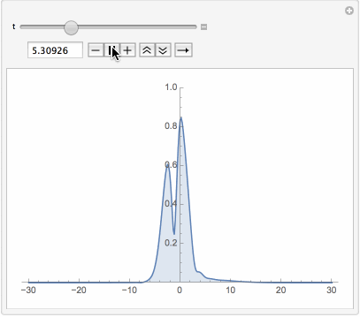
Manipulate[Plot[Evaluate[Abs[u[t, x] /. First[sol]]], {x, -L, L},
  PlotPoints -> 40, PlotRange -> {0, 1}, Filling -> Bottom], {t, 0, T}]


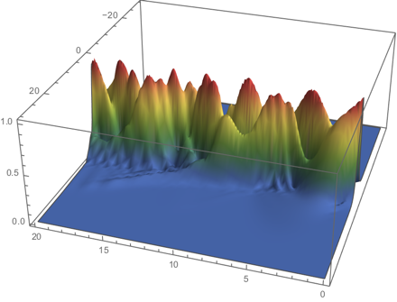
Plot3D[Evaluate[Abs[u[t, x] /. First[sol]]], {t, 0, T}, {x, -L, L},
PlotPoints -> 60, Mesh -> None, PlotRange -> All, ColorFunction -> "DarkRainbow"]


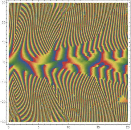
DensityPlot[Evaluate[Arg[u[t, x] /. First[sol]]], {t, 0, T}, {x, -L, L},
PlotPoints -> 60, MaxRecursion -> 3, ColorFunction -> "DarkRainbow"]

POSTED BY: Vitaliy Kaurov
One of the big advantages of Mathematica's notebook interface is that you can look at intermediate results.
When I ran the NDSolve step I got a warning:
NDSolve::bcart: Warning: an insufficient number of boundary conditions have been specified for the direction of independent variable x. Artificial boundary effects may be present in the solution. >>
If I plot Pl[x,0], I get a function strongly peaked at the origin.  If I plot P[x,1]  I get a function going up to 10^70 at x = -10 and 10.
If you replace the Animate step with
Manipulate[Plot[P[x,t],{x,-10,10},PlotRange -> All],{t,0,10}]
you can see that.
POSTED BY: Frank Kampas
Posted 11 years ago
A little new update:
 V[x_, t_] = Evaluate[Input["Enter the potential function:", Abs[x]]];
 m = Evaluate[Input["Enter the mass of the particle:", 1]];
 collapsePower = 5;
 collapseWidth = 1/1000
 collapseX = 0
 h = 6.62606957*10^-34;
 hbar = h/(2*\[Pi]);
 \[Psi][x_] = collapseX + 1/(Abs[x/collapseWidth]^collapsePower + 1);
 \[Psi]n[x_] = \[Psi][x]/
   NIntegrate[\[Psi][x], {x, -Infinity, Infinity}];
S = NDSolve[{I*hbar*
      D[\[CapitalPsi][x, t], t] == -hbar^2/(2*m)*
       Laplacian[\[CapitalPsi][x, t], {x}] + V[x, t], \[CapitalPsi][x,
       0] == \[Psi]n[x]}, \[CapitalPsi], {x, -10, 10}, {t, 0, 10}];
P[x_, t_] = Abs[\[CapitalPsi][x, t] /. S]^2;
Animate[Plot[{P[x, t], V[x, t]}, {x, -10, 10}, PlotRange -> 10], {t,
  0, 10}, AnimationRunning -> True]

But the problem is there still.
POSTED BY: Max Fischer
Posted 11 years ago
Now i have constructed code with NDSolve:
 V[x_] = Evaluate[Input["Enter the potential function:", Abs[x]]];
 m = Evaluate[Input["Enter the mass of the particle:", 1]];
 collapsePower = 5;
 collapseWidth = 1/1000
 collapseX = 0
 h = 6.62606957*10^-34;
 hbar = h/(2*\[Pi]);
 \[Psi][x_] = collapseX + 1/(Abs[x/collapseWidth]^collapsePower + 1);
 \[Psi]n[x_] = \[Psi][x]/
   N[Integrate[\[Psi][x], {x, -Infinity, Infinity}]];
S = NDSolve[{I*hbar*
      D[\[CapitalPsi][x, t], t] == -hbar^2/(2*m)*
       Laplacian[\[CapitalPsi][x, t], {x}] + V[x], \[CapitalPsi][x,
      0] == \[Psi]n[x]}, \[CapitalPsi], {x, -10, 10}, {t, 0, 10}];
P[x_, t_] = Abs[\[CapitalPsi][x, t] /. S]^2;
Animate[Plot[P[x, t], {x, -10, 10}, PlotRange -> 1], {t, 0, 10},
AnimationRunning -> True]
But it does not view any graph
POSTED BY: Max Fischer
Did DSolve evaluate?  Most differential equations cannot be solved in closed form.
Maybe NDSolve would work.
POSTED BY: Frank Kampas
Posted 11 years ago
I have edited the code and removed a lot of bugs, but the problem is there still: It would not plot the wave function.
POSTED BY: Max Fischer
There appears to be a few syntax errors here. I think you need to look in the manual for how to define functions..You can test each function after you've defined it: if Psi doesn't work then nothing that comes after it will work. Also, if you remove the semicolons you'll notice errors better. (The semicolon after your Animate suppresses the animation altogether!) 

As Frank says, your function:
\[CapitalPsi][x_, t_] := D[\[CapitalPsi][x, t], t] == -hbar^2/(2*m)* Laplacian[\[CapitalPsi][x, t], {x}] + v[x], \[CapitalPsi][x,
    0] == \[Psi]n[x]}, \[CapitalPsi], {x, t}]
doesn't work - for me it's generating recursion depth errors when called, it appears to be calling itself? 

In the previous line before this there appear to be too many x's, giving the error "raw object cannot be used an an iterator". 
It might be an idea to find a Mathematica tutorial and build some more straightforward functions and animations first. Then move on to quantum stuff when you're ready...
POSTED BY: C ormullion
If you look at \[x,t], you'll see that DSolve didn't evaluate its input.
POSTED BY: Frank Kampas
I tried to copy capital psi[x,t] into the window but the capital psi didn't get there.
POSTED BY: Frank Kampas
Reply to this discussion
Community posts can be styled and formatted using the Markdown syntax.
Reply Preview
Attachments
Remove
or Discard

Group Abstract Group Abstract